Heat Waves - AIFS - Open Data Visio

In the end of April 2025, Western European countries experienced unseasonably warm weather. This example shows analysis of the selected parameters:

z geopotential at constant pressure level 500 hPa,
t temperature at 850 hPa, and
2t 2 metre temperature of the AIFS-Single datasets on 30 April at 12 UTC in France (48.3° N, 4.1° E).

1. Set Up Your Environment and Find ECMWF Open Data¶

Open data will be downloaded from a publicly available Amazon S3 Bucket. First, the following Python libraries need to be installed in the current Jupyter kernel:

ecmwf-opendata to download data and
earthkit to analyse and plot the data.

If the packages are not installed yet, uncomment the code below and run it.

# !pip3 install earthkit ecmwf-opendata

from ecmwf.opendata import Client
import earthkit.data as ekd
import earthkit.plots as ekp
import earthkit

List of parameters to retrieve from open datasets¶

The selected values below can be modified.

Parameters available on pressure levels:

PARAM_PL = ["z", "t"]
LEVELS = [500, 850]
LEVELTYPE = "pl"

DATES = [20250429, 20250430, 20250501]
TIME = 0
STEPS = 12
STREAM = "oper"
TYPE = "fc"
MODEL = "aifs-single"

Parameters available on a single level:

PARAM_SFC = ["2t"]
LEVELTYPE = "sfc"

DATES = [20250429, 20250430, 20250501]
TIME = 0
STEPS = 12
STREAM = "oper"
TYPE = "fc"
MODEL = "aifs-single"

Get the data using the ECMWF Open Data API¶

def get_open_data(date, time, step, stream, _type, model, param, leveltype, levelist=[]):
    client = Client(source="aws")
    list_of_files = []
    # Get the data for all dates
    for _date in DATES:
        filename = f"{model}_{''.join(param)}_{''.join(map(str, levelist))}_{_date}.grib2" if levelist else f"{model}_{''.join(param)}_{leveltype}_{_date}.grib2"
        data = client.retrieve(
            date=_date,
            time=time,
            step=step,
            stream=stream,
            type=_type,
            levtype=leveltype,
            levelist=levelist,
            param=param,
            model=model,
            target=filename
            )
        list_of_files.append(filename)
    return data, list_of_files

2. Geopotential at 500 hPa and temperature at 850 hPa¶

When using the ls() method, a list of all the fields in the file we downloaded will be displayed.

data, list_of_files = get_open_data(date=DATES,
                                    time=TIME,
                                    step=STEPS,
                                    stream=STREAM,
                                    _type=TYPE,
                                    model=MODEL,
                                    param=PARAM_PL,
                                    leveltype=LEVELTYPE,
                                    levelist=LEVELS)

# Select AIFS model data from 29 April 2025
ds = ekd.from_source("file", list_of_files[0])
ds.ls()

Only the parameters and their levels which we specified above will be returned when we apply the sel() function.

t850 = ds.sel({"level": 850, "shortName": "t"})
t850.ls()

In the cell below, the geopotential on 500 hPa is selected and a new fieldlist with a single field containing the new values and metadata is created.

z500 = ds.sel({"level": 500, "shortName": "z"})[0]
z500.ls()

Important

For single fields, one has to use the bracket operator to fetch the first element from a list and access as well as modify its metadata:

ds.sel({"level": 500, "shortName": "z"}) # MaskIndex(GRIBReader(aifs-single_zt_500850_20250429.grib2),[2])
ds.sel({"level": 500, "shortName": "z"})[0] # GribField(z,500,20250429,0,12,None)

To change metadata values, put key value pairs to the override() function.

md_gh500 = z500.metadata().override(shortName="gh")
md_gh500["shortName"], md_gh500["level"]

('gh', 500)

Geopotential height is calculated by dividing the geopotential by the Earth’s mean gravitational acceleration, g (=9.80665 m s-2). In the ECMWF Open Charts, it is plotted in geopotential decameters. Therefore, our result also need to be divided by 10.

ds_gh500 = z500.values / (9.80665 * 10)
gh500 = ekd.FieldList.from_array(ds_gh500, md_gh500)
gh500.ls()

3. 2-metre temperature¶

The input values can be set here.

data, list_of_files = get_open_data(date=DATES,
                                    time=TIME,
                                    step=STEPS,
                                    stream=STREAM,
                                    _type=TYPE,
                                    model=MODEL,
                                    param=PARAM_SFC,
                                    leveltype=LEVELTYPE,
                                    levelist=[])

# Select data from 30 April 2025
ds_2t = ekd.from_source("file", list_of_files[1])
ds_2t.ls()

There is no need to convert temperature from Kelvin to Celsius, because in the earthkit-plots library we can set units of it.

t2m = ds_2t.sel(shortName="2t")
t2m.ls()

4. Data visualisation¶

The plot below shows analysis of T850 and z500 on 29 April 2025.

chart = ekp.Map(domain="Europe")

t850_shade = ekp.styles.Style(
    colors="Spectral_r",
    levels=range(-40, 50, 2),
    units="celsius",
)

chart.grid_cells(t850, style=t850_shade)
chart.contour(gh500, legend_style="None")

chart.coastlines(resolution="low")
chart.gridlines()

chart.legend(location="bottom", label="{variable_name} ({units})")

chart.title(
    "AIFS-Single: 500 hPa geopotential height and 850 hPa temperature\n"
    "{base_time:%Y-%m-%d %H} UTC (+{lead_time}h)\n",
    fontsize=14, horizontalalignment="center",
)
chart.save(f"./plots/{''.join(PARAM_PL)}_{MODEL}_{DATES[0]}{TIME}-{STEPS}h.png")
chart.show()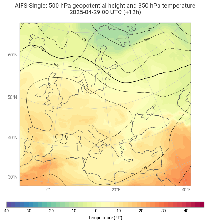

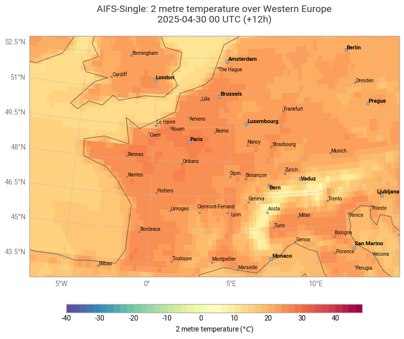
The plot below show analysis of 2 metre temperature on 30 April at 00 UTC.

chart = ekp.Map(domain=[-7, 15, 43, 53])

t2m_shade = ekp.styles.Style(
    colors="Spectral_r",
    levels=range(-40, 50, 2),
    units="celsius",
)

chart.grid_cells(t2m, style=t2m_shade)

chart.title(
    "AIFS-Single: {variable_name} over Western Europe\n"
    "{base_time:%Y-%m-%d %H} UTC (+{lead_time}h)\n",
    fontsize=14, horizontalalignment="center",
)

chart.coastlines(resolution="low")
chart.gridlines()
chart.cities(adjust_labels=True)

chart.legend(location="bottom", label="{variable_name} ({units})")

chart.save(f"./plots/{''.join(PARAM_SFC)}_{MODEL}_{DATES[1]}{TIME}-{STEPS}h.png")
chart.show()