Heat Waves - IFS - Open Data Visio

Here we will focus on:

2t 2 metre temperature,
mn2t3 minimum temperature at 2 metres in the last 3 hours, and
mx2t3 maximum temperature at 2 metres in the last 3 hours in France on 30 April at 12 UTC.

1. Set Up Your Environment and Find ECMWF Open Data¶

If the packages are not installed yet, uncomment the code below and run it.

# !pip3 install earthkit ecmwf-opendata

from ecmwf.opendata import Client
import earthkit.data as ekd
import earthkit.plots as ekp

List of parameters to retrieve from open datasets¶

The selected values below can be modified.

PARAM_SFC = ["mn2t3", "mx2t3", "2t"]
PARAM_PL = []
LEVELS = []
LEVELTYPE = "sfc"

DATES = [20250429, 20250430, 20250501]
TIME = 0
STEPS = 12
STREAM = "oper"
TYPE = "fc"
MODEL = "ifs"

Get the data using the ECMWF Open Data API¶

def get_open_data(date, time, step, stream, _type, model, param, leveltype, levelist=[]):
    client = Client(source="aws")
    list_of_files = []
    # Get the data for all dates
    for _date in DATES:
        filename = f"{model}_{''.join(param)}_{''.join(map(str, levelist))}_{_date}.grib2" if levelist else f"{model}_{''.join(param)}_{leveltype}_{_date}.grib2"
        data = client.retrieve(
            date=_date,
            time=time,
            step=step,
            stream=stream,
            type=_type,
            levtype=leveltype,
            levelist=levelist,
            param=param,
            model=model,
            target=filename
            )
        list_of_files.append(filename)
    return data, list_of_files

2. 2-metre temperature¶

The input values can be set here.

data, list_of_files = get_open_data(date=DATES,
                                    time=TIME,
                                    step=STEPS,
                                    stream=STREAM,
                                    _type=TYPE,
                                    model=MODEL,
                                    param=PARAM_SFC,
                                    leveltype=LEVELTYPE,
                                    levelist=[])

# Select data from 30 April 2025
ds_2t = ekd.from_source("file", list_of_files[1])
ds_2t.ls()

When using the describe() method, a given parameter defined by shortName will be described.

t2m = ds_2t.sel(shortName="2t")
t2m.describe("2t")

Important

One has to use the bracket operator to fetch the first element from a list and inspect its namespaces:

ds_2t.sel(shortName="mx2t3") # MaskIndex(GRIBReader(ifs_mn2t3mx2t32t_sfc_20250430.grib2),[0])
ds_2t.sel(shortName="mx2t3")[0] # GribField(mx2t3,None,20250430,0,12,None)

The dump() method inspects all the namespace keys of a parameter.
By clicking on different tabs below, the content of various namespaces will be displayed.

t2max_K = ds_2t.sel(shortName="mx2t3")[0]
t2max_K.dump()

md_t2max = t2max_K.metadata()
ds_t2max = t2max_K.values - 273.15
t2max = ekd.FieldList.from_array(ds_t2max, md_t2max)
t2max.ls()

t2min_K = ds_2t.sel(shortName="mn2t3")
t2min_K.metadata("units")[0]

'K'

md_t2min = t2min_K.metadata()
ds_t2min = t2min_K.values - 273.15
t2min = ekd.FieldList.from_array(ds_t2min, md_t2min)
t2min.ls()

3. Data visualisation¶

We will plot our data from IFS on the map defining our specific plotting methods.

IFS¶

The plots below show analyses of 2 metre temperature, minimum, and maximum temperature at 2 metres in the last 3 hours on 30 April at 00 UTC.

chart = ekp.Map(domain=[-7, 15, 43, 53])

t2m_shade = ekp.styles.Style(
    colors="Spectral_r",
    levels=range(-40, 50, 2),
    units="celsius",
)

chart.grid_cells(t2m, style=t2m_shade)

chart.title(
    "IFS: {variable_name} over Western Europe\n"
    "{base_time:%Y-%m-%d %H} UTC (+{lead_time}h)\n",
    fontsize=14, horizontalalignment="center",
)

chart.coastlines(resolution="low")
chart.gridlines()
chart.cities(adjust_labels=True)

chart.legend(location="bottom", label="{variable_name} ({units})")

chart.save(f"./plots/{PARAM_SFC[-1]}_{MODEL}_{DATES[1]}{TIME}-{STEPS}h.png")
chart.show()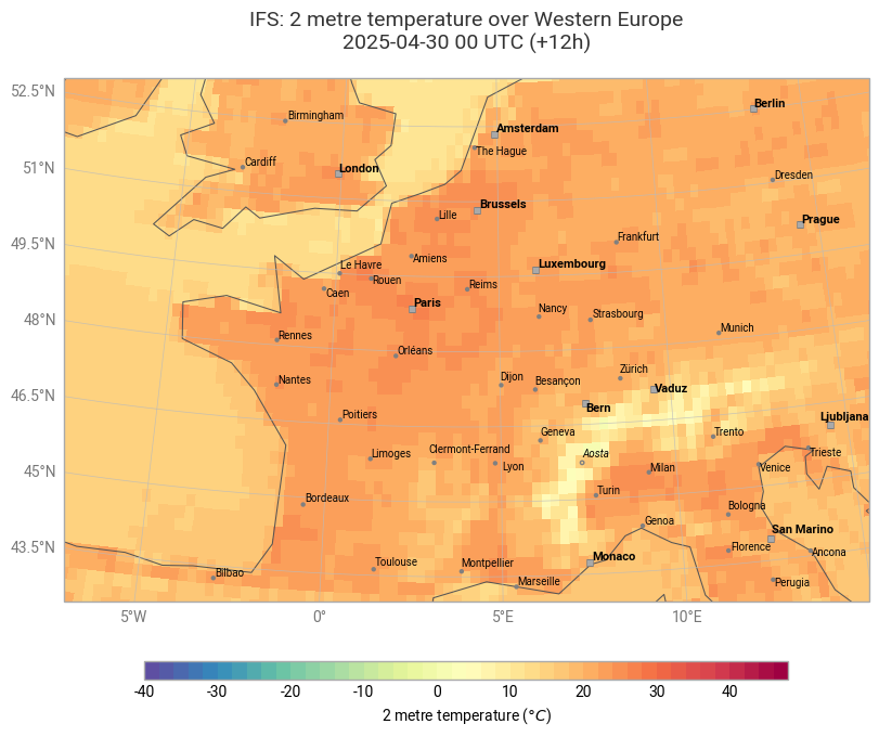

figure = ekp.Figure(domain="France", size=(9, 7), rows=1, columns=2)

t2maxmin_shade = ekp.styles.Style(
    colors="Spectral_r",
    levels=range(0, 32, 2),
)

figure.contourf(t2max, style=t2maxmin_shade)
subplot = figure.add_map(0, 1)
subplot.contourf(t2min, style=t2maxmin_shade)

figure.title("IFS: {variable_name} over {domain}\n {base_time:%Y-%m-%d %H} UTC (+{lead_time}h)")

figure.coastlines(resolution="low")
figure.gridlines()

figure.legend(location="bottom", label="Temperature (˚C)")

figure.save(fname=f"./plots/{''.join(PARAM_SFC[0:2])}_{MODEL}_{DATES[1]}{TIME}-{STEPS}h.png")
figure.show()

<Figure size 900x700 with 0 Axes>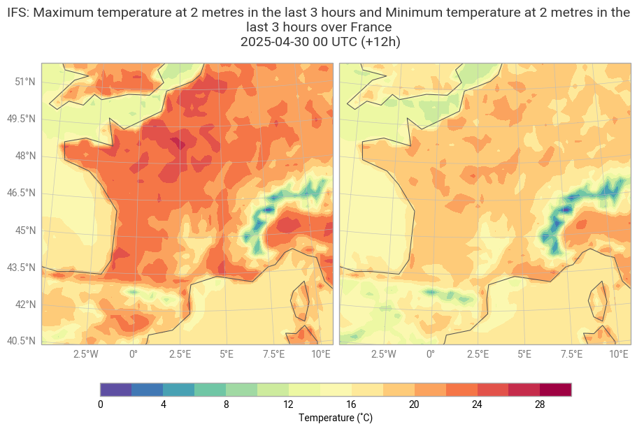

IFS Control Forecast¶

In the short-range forecasts on 30 April 2025, one can see the sign of a heat-island over Paris and London.

PARAM_SFC = "2t"
PARAM_PL = []
LEVELS = []
LEVELTYPE = "sfc"

DATES = 20250430
TIME = 12
STEPS = [0, 48, 72, 120]
STREAM = "enfo"
TYPE = "cf"
MODEL = "ifs"

filename = f"{MODEL}_{PARAM_SFC}_{DATES}_{'-'.join(map(str, STEPS))}.grib2"

def get_open_data_Nsteps(filename, date, time, step, stream, _type, model, param, leveltype, levelist=[]):
    client = Client(source="aws")
    # Get the data for all steps
    data = client.retrieve(
        date=date,
        time=time,
        step=step,
        stream=stream,
        type=_type,
        levtype=leveltype,
        levelist=levelist,
        param=param,
        model=model,
        target=filename
        )
    return data

data = get_open_data_Nsteps(filename,
                            date=DATES,
                            time=TIME,
                            step=STEPS,
                            stream=STREAM,
                            _type=TYPE,
                            model=MODEL,
                            param=PARAM_SFC,
                            leveltype=LEVELTYPE,
                            levelist=[])

ds_ifs = ekd.from_source("file", filename)
t2m_ifs = ds_ifs.sel(shortName="2t")
t2m_ifs.ls()

figure = ekp.Figure(domain=[-7, 15, 43, 53], size=(9, 9), rows=2, columns=4)

t2mifs_shade = ekp.styles.Style(
    colors="Spectral_r",
    levels=range(-40, 50, 2),
    units="celsius",
)

for i in range(4):
    figure.add_map(1+i//4, i%4)

figure.contourf(t2m_ifs, style=t2mifs_shade)

figure.coastlines()
figure.gridlines()

figure.legend(label="{variable_name} ({units})")

figure.subplot_titles("{base_time:%Y-%m-%d %H} UTC (+{lead_time}h)")
figure.title(
    "IFS (Control Forecast): {base_time:%Y-%m-%d %H} UTC\n {variable_name} over Western Europe\n\n",
    fontsize=14, horizontalalignment="center",
)
figure.save(fname=f"./plots/{PARAM_SFC}_{MODEL}_{DATES}{TIME}-{'-'.join(map(str, STEPS))}h.png")
figure.show()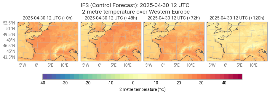

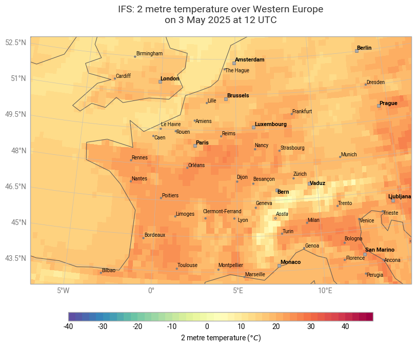
Compared to the IFS Control Forecast, one can note that the event was well captured by the IFS model from 30 April and onwards.

filename_fc="ifs_2t_20250503120000-0h.grib2"

client = Client(source="aws")
client.retrieve(
    date=20250503,
    time=12,
    step=0,
    stream="oper",
    type="fc",
    levtype="sfc",
    param='2t',
    model="ifs",
    target=filename_fc
)

<ecmwf.opendata.client.Result at 0x7cfd8efe0f20>

ds_fc = ekd.from_source("file", filename_fc)
t2m_fc = ds_fc.sel(shortName="2t")
t2m_fc.ls()

chart = ekp.Map(domain=[-7, 15, 43, 53])

t2mfc_shade = ekp.styles.Style(
    colors="Spectral_r",
    levels=range(-40, 50, 2),
    units="celsius",
)

chart.grid_cells(t2m_fc, style=t2mfc_shade)

chart.title(
    "IFS: {variable_name} over Western Europe\n"
    "on {time:%-d %B %Y at %H UTC}\n",
    fontsize=14, horizontalalignment="center",
)
chart.coastlines(resolution="low")
chart.gridlines()
chart.cities(adjust_labels=True)

chart.legend(location="bottom", label="{variable_name} ({units})")

chart.save("./plots/ifs_2t_20250503120000-0h.png")
chart.show()