Tropical Cyclone - Open Data Visio

At the end of February 2025, the tropical cyclone Honde affected the southern coast of Madagascar. It caused very heavy rainfall and strong winds.

This example shows analysis of the selected parameter:

tc tropical cyclone trajectory of the IFS datasets on 28 February at 00 UTC in Madagascar (22.95° S, 44.1° E).

1. Set Up Your Environment and Find ECMWF Open Data¶

Open data will be downloaded from a publicly available Amazon S3 Bucket. First, the following Python libraries need to be installed in the current Jupyter kernel:

ecmwf-opendata to download data,
earthkit to analyse and plot the data,
matplotlib to create visualizations, and
cartopy for cartographic visualizations.

If the packages are not installed yet, uncomment the code below and run it.

# !pip3 install earthkit ecmwf-opendata matplotlib cartopy

from ecmwf.opendata import Client
import earthkit.data as ekd

import matplotlib.pyplot as plt
import cartopy.crs as ccrs
import cartopy.feature as cfeature

import os

List of parameters to retrieve from open datasets¶

The selected values below can be modified.

PARAM_SFC = ["tc"]
LEVELTYPE = "sfc"

DATES = [20250228, 20250301]
TIME = 0
STEPS = 240
STREAM = "oper"
TYPE = "tf"
MODEL = "ifs"

Data and plots directories¶

DATADIR = './data_dir/'
os.makedirs(DATADIR, exist_ok=True)

PLOTSDIR = './plots/'
os.makedirs(PLOTSDIR, exist_ok=True)

Get the data using the ECMWF Open Data API¶

def get_open_data(date, time, step, stream, _type, model, param, leveltype, levelist=[]):
    client = Client(source="aws")
    list_of_files = []
    # Get the data for all dates
    for _date in DATES:
        filename = f"{DATADIR}{model}_{''.join(param)}_{''.join(map(str, levelist))}_{_date}.grib2" if levelist else f"{DATADIR}{model}_{''.join(param)}_{leveltype}_{_date}.grib2"
        data = client.retrieve(
            date=_date,
            time=time,
            step=step,
            stream=stream,
            type=_type,
            levtype=leveltype,
            levelist=levelist,
            param=param,
            model=model,
            target=filename
            )
        list_of_files.append(filename)
    return data, list_of_files

2. Tropical cyclone tracks and pressure reduced to mean sea level¶

When using the ls() method, metadata from the header section of the BUFR we downloaded will be displayed.

data, list_of_files = get_open_data(date=DATES,
                                    time=TIME,
                                    step=STEPS,
                                    stream=STREAM,
                                    _type=TYPE,
                                    model=MODEL,
                                    param=PARAM_SFC,
                                    leveltype=LEVELTYPE,
                                    levelist=[])

# Select AIFS model data from 28 February 2025
ds = ekd.from_source("file", list_of_files[0])
ds.ls()

df = ds.to_pandas(columns=["stormIdentifier", "latitude", "longitude", "pressureReducedToMeanSeaLevel"])
df

The column stormIdentifier contains ID numbers of different storms in the BUFR file.

df["stormIdentifier"].unique()

array(['10S', '11S', '18P', '21P'], dtype=object)

In this case study we will analyse the tropical cyclone Honde, thus we will select stormIdentifier=11S.

tc_h = df[df["stormIdentifier"] == '11S']
tc_h.head()

We will plot pressure reduced to mean sea level data in hPa, therefore we need to divide them by 100.

pmsl = tc_h["pressureReducedToMeanSeaLevel"] / 100
pmsl

13     969.0
14     971.0
15     971.0
16     970.0
17     970.0
18     973.0
19     973.0
20     975.0
21     976.0
22     978.0
23     978.0
24     980.0
25     980.0
26     980.0
27     978.0
28     977.0
29     975.0
30     976.0
31     973.0
32     975.0
33     974.0
34     980.0
35     981.0
36     984.0
37     985.0
38     989.0
39     991.0
40     996.0
41     998.0
42    1003.0
43    1005.0
44    1009.0
Name: pressureReducedToMeanSeaLevel, dtype: float64

3. 10 metre wind speed¶

Here we will retrieve data from the IFS Ensemble.
The input values can be set here.

PARAM_SFC = ["tc"]
LEVELTYPE = "sfc"

DATES = [20250228]
TIME = 0
STEPS = 240
STREAM = "enfo"
TYPE = "tf"
MODEL = "ifs"

data, list_of_files = get_open_data(date=DATES,
                                    time=TIME,
                                    step=STEPS,
                                    stream=STREAM,
                                    _type=TYPE,
                                    model=MODEL,
                                    param=PARAM_SFC,
                                    leveltype=LEVELTYPE,
                                    levelist=[])

# Select AIFS model data from 28 February 2025
ds_ens = ekd.from_source("file", list_of_files)
ds_ens

df_ens = ds_ens.to_pandas(columns=["stormIdentifier", "ensembleMemberNumber", "latitude", "longitude", "windSpeedAt10M"])
df_ens

After selecting stormIdentifier=11S, we will remove the column stormIdentifier from our Pandas DataFrame.

tc_h_ens = df_ens[df_ens["stormIdentifier"] == '11S']
tc_h_ens = tc_h_ens.drop('stormIdentifier', axis=1)
tc_h_ens

First we will sort the data according to their ensemble member numbers and then we will calculate the mean of them.

tc_h_ens = tc_h_ens.dropna(axis=0)
tc_h_ens = tc_h_ens.sort_values('ensembleMemberNumber')
tc_h_ens = tc_h_ens.drop('ensembleMemberNumber', axis=1)
mean_ens = tc_h_ens.groupby(['latitude', 'longitude'], as_index=False, dropna=True).mean()
mean_ens

4. Data visualisation¶

The plots below show the tropical cyclone track for TC Honde and the analysis of pressure reduced to mean sea level on 28 February 2025.

fig, (ax1, ax2) = plt.subplots(nrows=2, subplot_kw={'projection': ccrs.PlateCarree()})

ax1.plot(tc_h["longitude"], tc_h["latitude"],
         color='red',
         label="Tropical cyclone track",
         linewidth=1,
         alpha=0.7,
         transform = ccrs.PlateCarree())
ax1.add_feature(cfeature.LAND, facecolor="#ffe2ab")
ax1.set_title("IFS: Tropical cyclone Honde along the south-western coast of Madagascar\n"
              f"{DATES[0]} 00 UTC (+{STEPS}h)",
              fontsize=14)
ax1.gridlines(draw_labels=True,
              linewidth=1,
              color='gray',
              alpha=0.5,
              linestyle='--') 
ax1.coastlines(color="#333333")
ax1.set_extent([42, 51, -26, -11], crs=ccrs.PlateCarree())
ax1.legend(loc="best", bbox_to_anchor=(2.1, 0., 0.5, 0.5))

ax2.plot(tc_h["longitude"], tc_h["latitude"],
         color='red',
         linewidth=1,
         alpha=0.7,
         transform = ccrs.PlateCarree())
ax2.add_feature(cfeature.LAND, facecolor="#ffe2ab")
ax2.gridlines(draw_labels=True,
              linewidth=1,
              color='gray',
              alpha=0.5,
              linestyle='--') 
ax2.coastlines(color="#333333")
ax2.set_extent([-180, 180, -90, 90], crs=ccrs.PlateCarree())

fig.savefig(f"{PLOTSDIR}{''.join(PARAM_SFC)}_{MODEL}_{DATES[0]}{TIME}-{STEPS}h.png", dpi=200, bbox_inches='tight')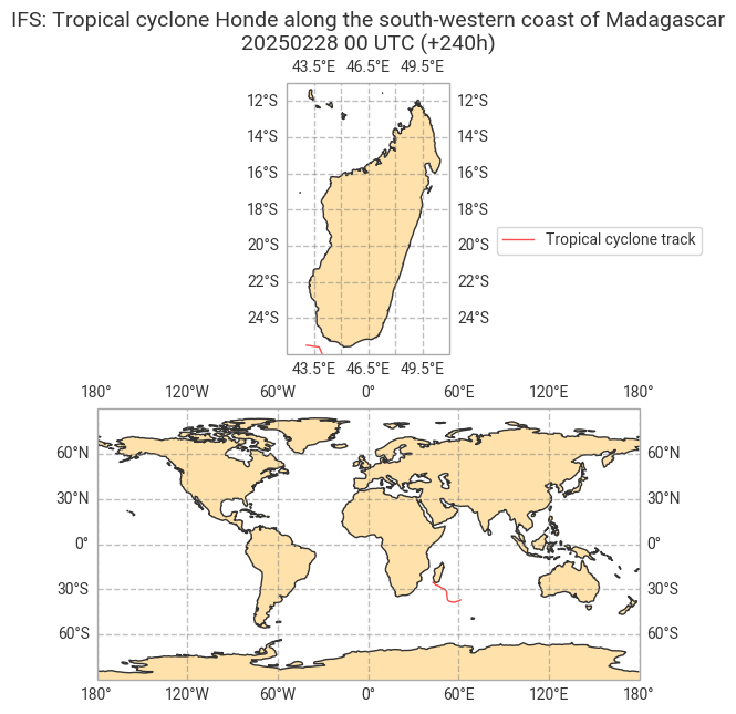

fig, (ax1, ax2) = plt.subplots(nrows=2, subplot_kw={'projection': ccrs.PlateCarree()})

pressure = ax1.scatter(tc_h.longitude, tc_h.latitude,
            s=100,
            c=pmsl,
            marker='o',
            cmap='viridis',
            alpha=0.9,
            edgecolors='face',
            transform = ccrs.PlateCarree(),
            zorder=10)
cbar = fig.colorbar(pressure, ax=ax1, pad=0.1)
cbar.set_label('Pressure (hPa)', fontsize=12)
ax1.set_title("IFS: Pressure reduced to mean sea level along the south-western coast of Madagascar\n"
              f"{DATES[0]} 00 UTC (+{STEPS}h)",
              fontsize=14)
ax1.add_feature(cfeature.LAND, facecolor="#ffe2ab")
ax1.gridlines(draw_labels=True,
              linewidth=1,
              color='gray',
              alpha=0.5,
              linestyle='--') 
ax1.coastlines(color="#333333")
ax1.set_extent([42, 51, -26, -11], crs=ccrs.PlateCarree())

ax2.scatter(tc_h["longitude"], tc_h["latitude"],
            s=10,
            c=pmsl,
            marker='o',
            cmap='viridis',
            alpha=0.9,
            edgecolors='face',
            transform = ccrs.PlateCarree(),
            zorder=10)
ax2.add_feature(cfeature.LAND, facecolor="#ffe2ab")
ax2.gridlines(draw_labels=True,
              linewidth=1,
              color='gray',
              alpha=0.5,
              linestyle='--') 
ax2.coastlines(color="#333333")
ax2.set_extent([-180, 180, -90, 90], crs=ccrs.PlateCarree())

fig.savefig(f"{PLOTSDIR}pmsl_{MODEL}_{DATES[0]}{TIME}-{STEPS}h.png", dpi=200, bbox_inches='tight')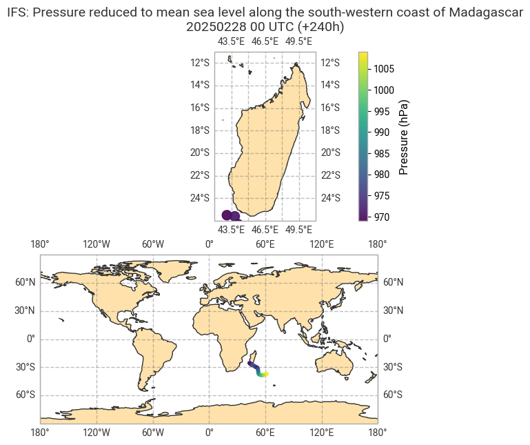

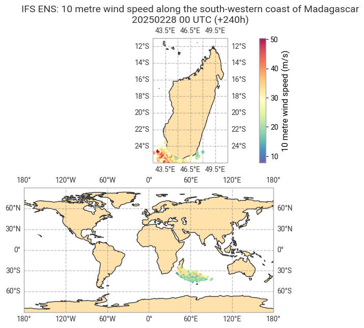
The plot below shows the analysis of 10 metre wind speed of the tropical cyclone Honde on 28 February 2025.

fig, (ax1, ax2) = plt.subplots(nrows=2, subplot_kw={'projection': ccrs.PlateCarree()})

ws10 = ax1.scatter(mean_ens["longitude"], mean_ens["latitude"],
            s=15,
            c=mean_ens.windSpeedAt10M,
            marker='o',
            cmap='Spectral_r',
            alpha=0.9,
            edgecolors='face',
            transform = ccrs.PlateCarree(),
            zorder=10)
cbar = fig.colorbar(ws10, ax=ax1, pad=0.1)
cbar.set_label('10 metre wind speed (m/s)', fontsize=12)
ax1.set_title("IFS ENS: 10 metre wind speed along the south-western coast of Madagascar\n"
              f"{DATES[0]} 00 UTC (+{STEPS}h)",
              fontsize=14)
ax1.add_feature(cfeature.LAND, facecolor="#ffe2ab")
ax1.gridlines(draw_labels=True,
              linewidth=1,
              color='gray',
              alpha=0.5,
              linestyle='--') 
ax1.coastlines(color="#333333")
ax1.set_extent([42, 51, -26, -11], crs=ccrs.PlateCarree())

ax2.scatter(mean_ens.longitude, mean_ens.latitude,
            s=5,
            c=mean_ens.windSpeedAt10M,
            marker='o',
            cmap='Spectral_r',
            alpha=0.9,
            edgecolors='face',
            transform = ccrs.PlateCarree(),
            zorder=10)
ax2.add_feature(cfeature.LAND, facecolor="#ffe2ab")
ax2.gridlines(draw_labels=True,
              linewidth=1,
              color='gray',
              alpha=0.5,
              linestyle='--') 
ax2.coastlines(color="#333333")
ax2.set_extent([-180, 180, -90, 90], crs=ccrs.PlateCarree())

fig.savefig(f"{PLOTSDIR}ws10_{MODEL}_{DATES[0]}{TIME}-{STEPS}h.png", dpi=200, bbox_inches='tight')