Cold Spells - AIFS - Open Data Visio

In the end of June 2025, South America experienced unprecedented cold temperatures. This example shows analysis of the selected parameters:

z geopotential at constant pressure level 500 hPa,
t temperature at 850 hPa,
sf snowfall, and
msl mean sea level pressure of the AIFS Ensemble datasets on 1 July at 06 UTC in Argentina (34.60° S, 58.38° W).

1. Set Up Your Environment and Find ECMWF Open Data¶

Open data will be downloaded from a publicly available Amazon S3 Bucket. First, the following Python libraries need to be installed in the current Jupyter kernel:

ecmwf-opendata to download data and
earthkit to analyse and plot the data.

If the packages are not installed yet, uncomment the code below and run it.

# !pip3 install earthkit ecmwf-opendata

from ecmwf.opendata import Client
import earthkit.data as ekd
import earthkit.plots as ekp
import earthkit

List of parameters to retrieve from open datasets¶

The selected values below can be modified.

Parameters available on pressure levels:

PARAM_PL = ["z", "t"]
LEVELS = [500, 850]
LEVELTYPE = "pl"

DATES = [20250701, 20250702]
TIME = 6
STEPS = 0
STREAM = "enfo"
TYPE = "cf"
MODEL = "aifs-ens"

Parameters available on a single level:

PARAM_SFC = ["sf", "msl"]
LEVELTYPE = "sfc"

DATES = [20250701, 20250702]
TIME = 6
STEPS = 6
STREAM = "enfo"
TYPE = "cf"
MODEL = "aifs-ens"

Get the data using the ECMWF Open Data API¶

def get_open_data(date, time, step, stream, _type, model, param, leveltype, levelist=[]):
    client = Client(source="aws")
    list_of_files = []
    # Get the data for all dates
    for _date in DATES:
        filename = f"{model}_{''.join(param)}_{''.join(map(str, levelist))}_{_date}.grib2" if levelist else f"{model}_{''.join(param)}_{leveltype}_{_date}.grib2"
        data = client.retrieve(
            date=_date,
            time=time,
            step=step,
            stream=stream,
            type=_type,
            levtype=leveltype,
            levelist=levelist,
            param=param,
            model=model,
            target=filename
            )
        list_of_files.append(filename)
    return data, list_of_files

2. Geopotential at 500 hPa and temperature at 850 hPa¶

When using the ls() method, a list of all the fields in the file we downloaded will be displayed.
The type cf indicates that we only retrieve the data of the control forecast.

data, list_of_files = get_open_data(date=DATES,
                                    time=TIME,
                                    step=STEPS,
                                    stream=STREAM,
                                    _type=TYPE,
                                    model=MODEL,
                                    param=PARAM_PL,
                                    leveltype=LEVELTYPE,
                                    levelist=LEVELS)

# Select AIFS model data from 1 July 2025
ds = ekd.from_source("file", list_of_files[0])
ds.ls()

We will use the sel() method to filter out the parameters and their levels that we do not want to analyse. The describe() method provides an overview of the selected parameter.

t850 = ds.sel({"level": 850, "shortName": "t"})
t850.describe("t")

z500 = ds.sel({"level": 500, "shortName": "z"})[0]
z500.ls()

Geopotential height is calculated by dividing the geopotential by the Earth’s mean gravitational acceleration, g (=9.80665 m s-2). In the ECMWF Open Charts, it is plotted in geopotential decameters. Therefore, our result also need to be divided by 10.

ds_gh500 = z500.values / (9.80665 * 10)

md_gh500 = z500.metadata().override(shortName="gh")
md_gh500["shortName"], md_gh500["level"]

('gh', 500)

gh500 = ekd.FieldList.from_array(ds_gh500, md_gh500)
gh500.ls()

3. Snowfall and mean sea level pressure¶

The input values can be set here.

data, list_of_files = get_open_data(date=DATES,
                                    time=TIME,
                                    step=STEPS,
                                    stream=STREAM,
                                    _type=TYPE,
                                    model=MODEL,
                                    param=PARAM_SFC,
                                    leveltype=LEVELTYPE,
                                    levelist=[])

# Select data from 1 July 2025
sf_msl = ekd.from_source("file", list_of_files[0])
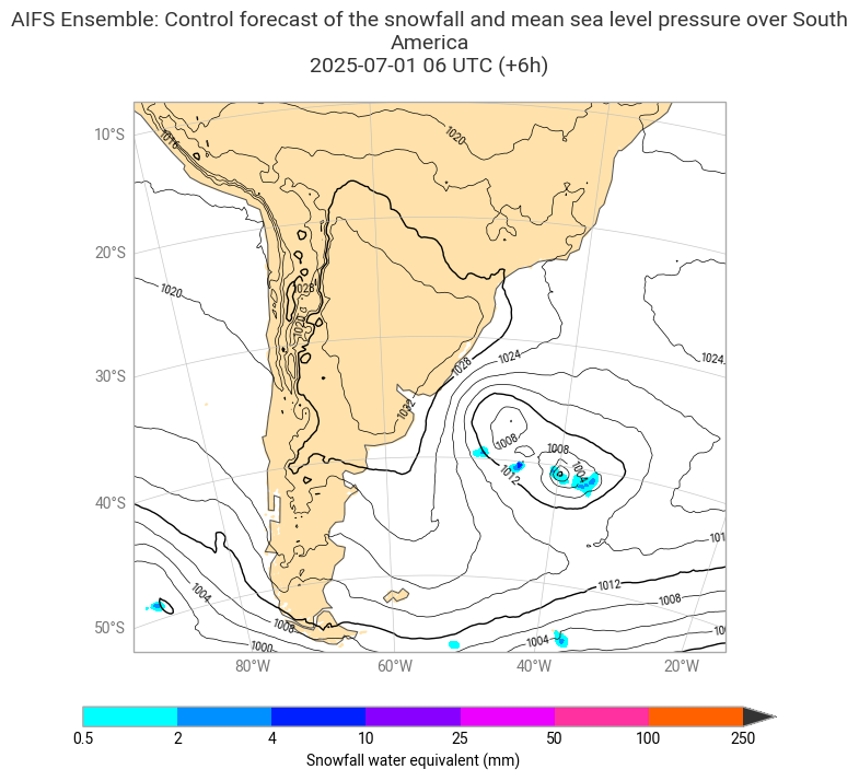
sf_msl.ls()

A unit of snowfall is kg/m $^2$ which corresponds to the snow depth 1 mm.
The sf parameter gives information about total snowfall from the start of the forecast onwards. For instance, step=6 indicates accumulated precipitation from 00 UTC until 06 UTC.

ds_sf = sf_msl.sel(shortName="sf")
ds_sf.describe("sf")

We will plot mean sea level pressure data in hPa, therefore we need to divide them by 100.

ds_msl = sf_msl.sel(shortName="msl")
ds_msl.describe("msl")

msl = ekd.SimpleFieldList()
md = ds_msl.metadata()
v = ds_msl.to_array() / 100
for f in range(len(md)):
    msl.append(ekd.ArrayField(v[f], md[f]))
msl.ls()

4. 2-metre temperature less than 273.15 K¶

The input values can be set here.

PARAM_SFC = ["2tl273"]
LEVELTYPE = "sfc"

DATES = [20250701]
TIME = 6
STEPS = 360
STREAM = "enfo"
TYPE = "ep"
MODEL = "aifs-ens"

To be continued

5. Data visualisation¶

The plot below shows analysis of T850 and z500 on 1 July 2025.

chart = ekp.Map(domain=[-80, -20, -55, -10])

t850_shade = ekp.styles.Style(
    colors="Spectral_r",
    levels=range(-40, 50, 2),
    units="celsius",
)

chart.contourf(t850, style=t850_shade)

chart.contour(gh500,
              levels={"step": 5, "reference": 550},
              linecolors="black",
              linewidths=[0.5, 1, 0.5, 0.5],
              labels = True,
              legend_style = None,
              transform_first=True)

chart.coastlines(resolution="low")
chart.gridlines()
chart.cities(capital_cities=True, adjust_labels=True)

chart.legend(location="right")

chart.title(
    "AIFS Ensemble: Control forecast of the 500 hPa geopotential height and 850 hPa temperature over South America\n"
    "{base_time:%Y-%m-%d %H} UTC (+{lead_time}h)\n",
    fontsize=14, horizontalalignment="center",
)
chart.save(f"./plots/{''.join(PARAM_PL)}_{MODEL}_{DATES[0]}{TIME}-{STEPS}h.png")
chart.show()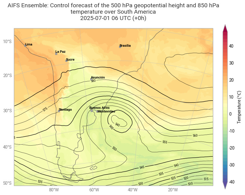

The plot below shows analysis of mean sea level pressure and snowfall on 1 July 2025.

chart = ekp.Map(domain=[-80, -30, -55, -10])

hex_colours = ['#00ffff', '#0080ff', '#0000ff', '#d900ff', '#ff00ff', '#ff8000', '#ff0000', '#333333', ]

sf_shade = ekp.styles.Style(
    colors = hex_colours,
    levels = [0.5, 2, 4, 10, 25, 50, 100, 250],
    extend = "max",
)

chart.land(color="#ffe2ab")
chart.contourf(ds_sf, style=sf_shade)
chart.contour(msl,
              levels={"step": 4, "reference": 1000},
              linecolors="black",
              linewidths=[0.5, 1, 0.5, 0.5],
              labels = True,
              legend_style = None,
              transform_first=True)

chart.coastlines(resolution="low")
chart.gridlines()

chart.legend(location="bottom", label="{variable_name} (mm)")

chart.title(
    "AIFS Ensemble: Control forecast of the snowfall and mean sea level pressure over South America\n"
    "{base_time:%Y-%m-%d %H} UTC (+{lead_time}h)\n",
    fontsize=14, horizontalalignment="center",
)
chart.save(f"./plots/{''.join(PARAM_SFC)}_{MODEL}_{DATES[0]}{TIME}-{STEPS}h.png")
chart.show()