High Winds - IFS - Open Data Visio

Here we will focus on:

10u 10 metre U wind component,
10v 10 metre V wind component,
10fg3 maximum 10 metre wind gust in the last 3 hours, and
10fgg15 10 metre wind gusts of at least 15 m/s of the IFS datasets on 7 January 2025 in Sweden (58.58° N, 11.07° E).

1. Set Up Your Environment and Find ECMWF Open Data¶

If the packages are not installed yet, uncomment the code below and run it.

# !pip3 install earthkit ecmwf-opendata xarray

from ecmwf.opendata import Client
import earthkit.data as ekd
import earthkit.plots as ekp

import xarray as xr
xr.set_options(keep_attrs=True)

<xarray.core.options.set_options at 0x7d46a4255d00>

List of parameters to retrieve from open datasets¶

The selected values below can be modified.

Parameters available on a single level:

PARAM_SFC = ["10u", "10v"]
LEVELTYPE = "sfc"

DATES = [20250107]
TIME = 0
STEPS = 0
STREAM = "enfo"
TYPE = ["cf", "pf"]
MODEL = "ifs"

To calculate the probabilities of 10 m wind speed, we need both the cf and pf type. This means that we will download the control forecast as well as all 50 ensemble members.
In case you want to download individual ensemble members, specify the type of data type=pf and the list of ensemble member numbers number=[1, 2, 3, ...].

Get the data using the ECMWF Open Data API¶

def get_open_data(date, time, step, stream, _type, model, param, leveltype, levelist=[]):
    client = Client(source="aws")
    list_of_files = []
    # Get the data for all dates
    for _date in DATES:
        filename = f"{model}_{''.join(param)}_{''.join(map(str, levelist))}_{_date}.grib2" if levelist else f"{model}_{''.join(param)}_{leveltype}_{_date}.grib2"
        data = client.retrieve(
            date=_date,
            time=time,
            step=step,
            stream=stream,
            type=_type,
            levtype=leveltype,
            levelist=levelist,
            param=param,
            model=model,
            target=filename
            )
        list_of_files.append(filename)
    return data, list_of_files

2. Wind speed probabilities¶

When using the ls() method, a list of all the fields in the file we downloaded will be displayed. Note that the ensemble member numbers are not sorted in an ascending or descending order.

data, list_of_files = get_open_data(date=DATES,
                                    time=TIME,
                                    step=STEPS,
                                    stream=STREAM,
                                    _type=TYPE,
                                    model=MODEL,
                                    param=PARAM_SFC,
                                    leveltype=LEVELTYPE,
                                    levelist=[])

# Select IFS model data from 7 January 2025
ds = ekd.from_source("file", list_of_files[0])
ds.ls()

The describe() method provides an overview of the selected parameter.

ds.describe("10u")

We will sort the ensemble member numbers (for 10u and 10v), then using the head() method, we will display the first 5 messages.

ds = ds.order_by(["number"])
ds.head()

We will calculate the wind speed from u and v components and create a new fieldlist with a single field containing new values. The metadata of the 10u field will be modified.

dsx = ds.to_xarray()
u = dsx['10u']
v = dsx['10v']
speed = xr.ufuncs.sqrt(u**2 + v**2)
speed = speed.assign_attrs(u.attrs)
speed.attrs['param'] = '10uv'
speed.attrs['standard_name'] = 'unknown'
speed.attrs['long_name'] = '10 metre wind speed'
speed.attrs['paramId'] = 'unknown'
speed

We will set values to 1 where the wind speed is higher than 10 m/s and to 0 where it is lower than 10 m/s.

speed01 = speed > 10

From there on we calculate the probability of the wind speed which is higher than 10 m/s, we calculate the mean of all the ensemble member numbers.

mean_ws = speed01.mean("number") * 100
mean_ws

The tail() method displays the last 5 messages when the n argument is not provided.

prob_ws = mean_ws.earthkit.to_fieldlist()
prob_ws.tail()

4. Wind gust¶

The input values can be set here.

PARAM_SFC = "10fg"
LEVELTYPE = "sfc"

DATES = [20250107]
TIME = 0
STEPS = 3
STREAM = "oper"
TYPE = "fc"
MODEL = "ifs"

When using the describe() method, a given parameter defined by shortName will be described.

data, list_of_files = get_open_data(date=DATES,
                                    time=TIME,
                                    step=STEPS,
                                    stream=STREAM,
                                    _type=TYPE,
                                    model=MODEL,
                                    param=PARAM_SFC,
                                    leveltype=LEVELTYPE,
                                    levelist=[])

# Select IFS model data on 7 January 2025
wg = ekd.from_source("file", list_of_files[0])
wg.describe("10fg")

5. 10 metre wind gusts of at least 15 m/s¶

The input values can be set here.

PARAM_SFC = ["10fgg15"]
LEVELTYPE = "sfc"

DATES = [20250107]
TIME = 0
STEPS = "0-24"
STREAM = "enfo"
TYPE = "ep"
MODEL = "ifs"

data, list_of_files = get_open_data(date=DATES,
                                    time=TIME,
                                    step=STEPS,
                                    stream=STREAM,
                                    _type=TYPE,
                                    model=MODEL,
                                    param=PARAM_SFC,
                                    leveltype=LEVELTYPE,
                                    levelist=[])

# Select data from 7 January 2025
wg15 = ekd.from_source("file", list_of_files[0])
wg15.ls()

6. Data visualisation¶

The plots below show analyses of 10 metre wind speed and direction and wind speed probabilities on 7 January 2025.

chart = ekp.Map(domain=[5, 23, 53, 65])

uv_style = ekp.styles.Style(
    colors="Spectral_r",
    levels=range(3, 10, 1),
    units="m/s",
)

chart.quiver(ds.sel(dataType="cf"), style=uv_style)

chart.coastlines(resolution="low")
chart.gridlines()
chart.cities(adjust_labels=True)

chart.legend(location="right", label="Wind speed ({units})")

chart.title(
    "IFS: Control forecast of 10 metre wind speed and direction over Southern Scandinavia\n"
    "{base_time:%Y-%m-%d %H} UTC (+{lead_time}h)\n",
    fontsize=14, horizontalalignment="center",
)
chart.save(f"./plots/{''.join(PARAM_SFC)}_{MODEL}_{DATES[0]}{TIME}-{STEPS}h.png")
chart.show()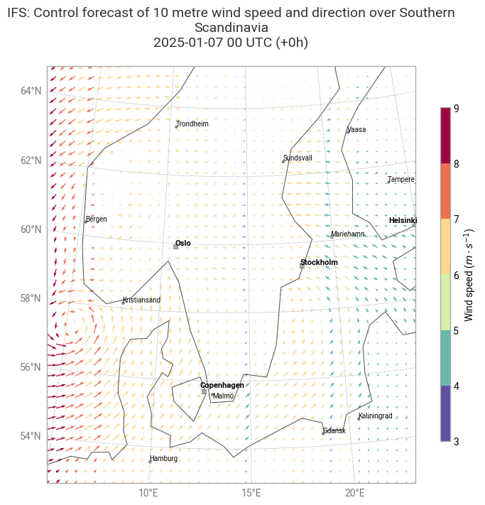

chart = ekp.Map(domain=[5, 23, 53, 65])

ws_style = ekp.styles.Style(
    colors="Spectral_r",
    levels=range(1, 100, 10),
    units="m/s",
)

chart.contourf(prob_ws, style=ws_style)

chart.coastlines(resolution="low")
chart.gridlines()
chart.cities(adjust_labels=True)

chart.legend(location="bottom", label="Wind speed ({units})")

chart.title(
    "IFS: Probability of 10 metre wind speed over Southern Scandinavia\n"
    "{base_time:%Y-%m-%d %H} UTC (+{lead_time}h)\n",
    fontsize=14, horizontalalignment="center",
)
chart.save(f"./plots/{''.join(PARAM_SFC)}_{MODEL}_{DATES[0]}{TIME}-{STEPS}h.png")
chart.show()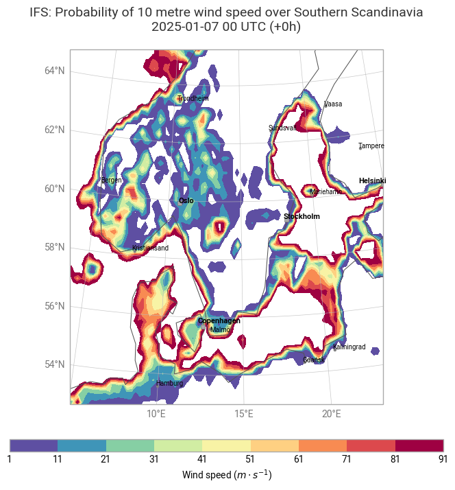

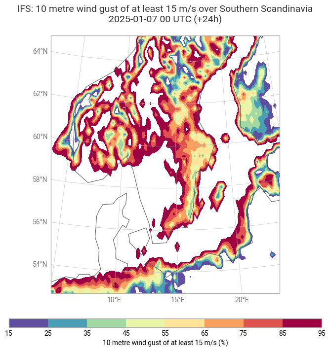
The plots below show analyses of maximum 10 metre wind gust in the last 3 hours and 10 metre wind gusts of at least 15 m/s on 7 January at 00 UTC.

chart = ekp.Map(domain=[5, 23, 53, 65])

wg_shade = ekp.styles.Style(
    colors="Spectral_r",
    levels=range(10, 50, 5),
    units="m/s",
    transform_first=True,
)

chart.contourf(wg, style=wg_shade)

chart.coastlines(resolution="low")
chart.gridlines()

chart.legend(location="bottom", label="{variable_name} ({units})")

chart.title(
    "IFS: 10m wind gust over Southern Scandinavia\n"
    "{base_time:%Y-%m-%d %H} UTC (+{lead_time}h)\n",
    fontsize=14, horizontalalignment="center",
)
chart.save(f"./plots/{PARAM_SFC}_{MODEL}_{DATES[0]}{TIME}-{STEPS}h.png")
chart.show()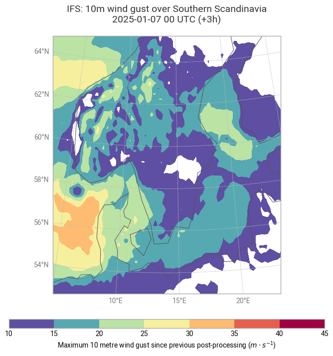

chart = ekp.Map(domain=[5, 23, 53, 65])

wg15_shade = ekp.styles.Style(
    colors="Spectral_r",
    levels=range(15, 100, 10),
    transform_first=True,
)

chart.contourf(wg15, style=wg15_shade)

chart.coastlines(resolution="low")
chart.gridlines()

chart.legend(location="bottom", label="{variable_name} (%)")

chart.title(
    "IFS: {variable_name} over Southern Scandinavia\n"
    "{base_time:%Y-%m-%d %H} UTC (+{lead_time}h)\n",
    fontsize=14, horizontalalignment="center",
)
chart.save(f"./plots/{''.join(PARAM_SFC)}_{MODEL}_{DATES[0]}{TIME}-{STEPS}h.png")
chart.show()