Winter storms had a tremendous impact on Sweden during the first week of January. A low-pressure system named Floriane impacted various parts of north-western Europe.
This example shows analysis of the selected parameters:
mslmean sea level pressure,tptotal precipitation of the AIFS datasets on 7 January 2025 in Sweden (58.58° N, 11.07° E).
1. Set Up Your Environment and Find ECMWF Open Data
Open data will be downloaded from a publicly available Amazon S3 Bucket. First, the following Python libraries need to be installed in the current Jupyter kernel:
requeststo send HTTP requests,itertoolsto create iterators for efficient looping,jsonto decode JSON data,xarrayto work with labelled multi-dimensional arrays, andearthkitto analyse and plot the data.
If the packages are not installed yet, uncomment the code below and run it.
# !pip3 install earthkit requests itertools json xarrayimport requests
import itertools
import json
import earthkit.data as ekd
import earthkit.plots as ekp
import earthkit
import os
import xarray as xr
xr.set_options(keep_attrs=True)<xarray.core.options.set_options at 0x733c097581d0>List of parameters to retrieve from open datasets
The selected values below can be modified.
Parameters available on a single level:
PARAM_SFC = "msl" # "tp"
LEVELTYPE = "sfc"

DATES = [20250104, 20250105, 20250106, 20250107, 20250108]
TIME = 0
STEPS = [24] # [12, 24]
STREAM = "oper"
TYPE = "fc"
MODEL = "aifs"
RESOL = "0p25"Data and plots directories
DATADIR = './data_dir/'
os.makedirs(DATADIR, exist_ok=True)

PLOTSDIR = './plots/'
os.makedirs(PLOTSDIR, exist_ok=True)
Get the data using the earthkit-data package
First we will extract information about the offset and length, byte ranges we want to read from a GRIB file.
def get_parts_index(date, time, step, stream, _type, model, resol, param, levelist=[]):
    """
    this function takes one parameter on a single level or a pressure level and
    returns its corresponding byte ranges extracted from the index file within a defined date range.
    """

    parts = []
    timez = f"{time}".zfill(2)

    for _date in DATES:
        for _step in STEPS:
            index = f"{_date}/{timez}z/{model}/{resol}/{stream}/{_date}{timez}0000-{_step}h-{stream}-{_type}.index"
            url = f"https://ecmwf-forecasts.s3.amazonaws.com/{index}"
            print(url)
            r = requests.get(url)
            r.raise_for_status()
            for i, line in enumerate(r.iter_lines()):
                line = json.loads(line)
                if levelist == []:
                    if line.get("param") == param:
                        offset = line["_offset"]
                        length = line["_length"]
                        parts.append((offset, length))
                else:
                    if line.get("levelist") == f"{levelist}" and line.get("param") == param:
                        offset = line["_offset"]
                        length = line["_length"]
                        parts.append((offset, length))
    return parts
def get_open_data_earthkit(date, time, step, stream, _type, model, resol, parts, scale):
files = ekd.SimpleFieldList()
timez = f"{time}".zfill(2)
# Get the data for all dates and steps
for _date in DATES:
for _step in STEPS:
filename = f"{DATADIR}{_date}/{timez}z/{model}/{resol}/{stream}/{_date}{timez}0000-{_step}h-{stream}-{_type}.grib2"
data = ekd.from_source("s3", {
"endpoint": "s3.amazonaws.com",
"region": "eu-central-1",
"bucket": "ecmwf-forecasts",
"objects": { "object": filename, "parts": parts.pop(0)},
}, anon=True)
md = data.metadata()
v = data.to_array() / scale
for f in range(len(md)):
files.append(ekd.ArrayField(v[f], md[f]))
return filesparts_pair = get_parts_index(date=DATES,
time=TIME,
step=STEPS,
stream=STREAM,
_type=TYPE,
model=MODEL,
resol=RESOL,
param=PARAM_SFC,
levelist=[])
parts_pairhttps://ecmwf-forecasts.s3.amazonaws.com/20250104/00z/aifs/0p25/oper/20250104000000-12h-oper-fc.index
https://ecmwf-forecasts.s3.amazonaws.com/20250104/00z/aifs/0p25/oper/20250104000000-24h-oper-fc.index
https://ecmwf-forecasts.s3.amazonaws.com/20250105/00z/aifs/0p25/oper/20250105000000-12h-oper-fc.index
https://ecmwf-forecasts.s3.amazonaws.com/20250105/00z/aifs/0p25/oper/20250105000000-24h-oper-fc.index
https://ecmwf-forecasts.s3.amazonaws.com/20250106/00z/aifs/0p25/oper/20250106000000-12h-oper-fc.index
https://ecmwf-forecasts.s3.amazonaws.com/20250106/00z/aifs/0p25/oper/20250106000000-24h-oper-fc.index
https://ecmwf-forecasts.s3.amazonaws.com/20250107/00z/aifs/0p25/oper/20250107000000-12h-oper-fc.index
https://ecmwf-forecasts.s3.amazonaws.com/20250107/00z/aifs/0p25/oper/20250107000000-24h-oper-fc.index
https://ecmwf-forecasts.s3.amazonaws.com/20250108/00z/aifs/0p25/oper/20250108000000-12h-oper-fc.index
https://ecmwf-forecasts.s3.amazonaws.com/20250108/00z/aifs/0p25/oper/20250108000000-24h-oper-fc.index
[(24225153, 845404),
(43801645, 941353),
(35521323, 845843),
(38581813, 942587),
(12135540, 846304),
(13769897, 945028),
(17586219, 722619),
(38844867, 816531),
(50391246, 843926),
(42232891, 814348)]ds = get_open_data_earthkit(date=DATES,
time=TIME,
step=STEPS,
stream=STREAM,
_type=TYPE,
model=MODEL,
resol=RESOL,
parts=parts_pair,
scale = 1) # Select AIFS model data from 4 to 8 January 2025
ds.ls()A unit of total precipitation is kg/m. 1 kg of rainwater fills an area of 1 m with the water of height 1 mm.
In the ECMWF Open Charts, total precipitation is also plotted in millimetres.
The tp parameter gives information about total accumulated rainfall from the start of the forecast onwards. For instance, step=12 indicates accumulated precipitation from 00 UTC until 12 UTC, step=24 from 00 UTC to 00 UTC on the next day.
To plot the total precipitation between the steps 12 and 24, we need the data on both timesteps and subtract the precipitation on step=24 from step=12.
tp_12 = ds.sel(step=12).to_xarray()
tp_24 = ds.sel(step=24).to_xarray()
tp24_12 = tp_24 - tp_12
tp = tp24_12.earthkit.to_fieldlist()
tp.ls()3. Mean sea level pressure
The input values can be set here.
We will plot mean sea level pressure data in hPa, therefore we need to divide them by 100.
parts_pair = get_parts_index(date=DATES,
                        time=TIME,
                        step=STEPS,
                        stream=STREAM,
                        _type=TYPE,
                        model=MODEL,
                        resol=RESOL,
                        param=PARAM_SFC,
                        levelist=[])
parts_pairhttps://ecmwf-forecasts.s3.amazonaws.com/20250104/00z/aifs/0p25/oper/20250104000000-24h-oper-fc.index
https://ecmwf-forecasts.s3.amazonaws.com/20250105/00z/aifs/0p25/oper/20250105000000-24h-oper-fc.index
https://ecmwf-forecasts.s3.amazonaws.com/20250106/00z/aifs/0p25/oper/20250106000000-24h-oper-fc.index
https://ecmwf-forecasts.s3.amazonaws.com/20250107/00z/aifs/0p25/oper/20250107000000-24h-oper-fc.index
https://ecmwf-forecasts.s3.amazonaws.com/20250108/00z/aifs/0p25/oper/20250108000000-24h-oper-fc.index
[(63582116, 476879),
 (18622014, 475416),
 (63177182, 473847),
 (31854527, 477943),
 (59839874, 479944)]
msl = get_open_data_earthkit(date=DATES,
time=TIME,
step=STEPS,
stream=STREAM,
_type=TYPE,
model=MODEL,
resol=RESOL,
parts=parts_pair,
scale = 100)
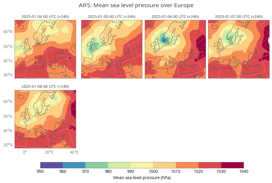
msl.ls()4. Data visualisation
The plots below show analyses of total precipitation and mean sea level pressure from 4 to 8 January 2025.
figure = ekp.Figure(domain="Europe", size=(9, 8), rows=3, columns=4)

hex_colours = ['#00ffff', '#0080ff', '#0000ff', '#d900ff', '#ff00ff', '#ff8000', '#ff0000', '#333333', ]

tp_shade = ekp.styles.Style(
    colors = hex_colours,
    levels = [0.5, 2, 4, 10, 25, 50, 100, 250],
    units = "mm",
    extend = "max",
)

for i in range(5):
    figure.add_map(1+i//4, i%4)
figure.contourf(tp, style=tp_shade)

figure.coastlines(resolution="low")
figure.gridlines()

figure.legend(location="bottom", label="{variable_name} ({units})")

figure.subplot_titles("{base_time:%Y-%m-%d %H} UTC (+12h, +24h)")
figure.title(
    "AIFS: {variable_name} over {domain}\n",
    fontsize=14, horizontalalignment="center",
)
figure.save(fname=f"{PLOTSDIR}{PARAM_SFC}_{MODEL}_{DATES[-1]}{TIME}-{STEPS[-1]}h.png")
figure.show()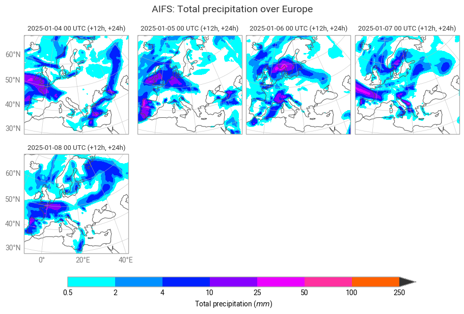
figure = ekp.Figure(domain="Europe", size=(9, 8), rows=3, columns=4)

msl_shade = ekp.styles.Style(
    colors="Spectral_r",
    levels=range(950, 1050, 10),
    extend="both",
    transform_first=True,
)

for i in range(5):
    figure.add_map(1+i//4, i%4)
figure.contourf(msl, style=msl_shade)

figure.coastlines(resolution="low")
figure.gridlines()

figure.legend(location="bottom", label="{variable_name} (hPa)")

figure.subplot_titles("{base_time:%Y-%m-%d %H} UTC (+{lead_time}h)")
figure.title(
    "AIFS: {variable_name} over {domain}\n",
    fontsize=14, horizontalalignment="center",
)
figure.save(fname=f"{PLOTSDIR}{PARAM_SFC}_{MODEL}_{DATES[-1]}{TIME}-{STEPS[-1]}h.png")
figure.show()