Chapter 4: Rising Seas#
Generation of plots based on the relevant Climate Indicators’ report.#
The ocean water in our planet covers over 70% of its surface, making it an ocean world. Not only that, but a large part of the global population resides near the coast, as does a lot of infrastructure and economic assets. Thus, although changes in sea level are a slow process, they can have a substantial impact in our future.
In this tutorial we will:
Search, download, and view data freely available in Climate Data Store and Copernicus Marine Service.
Use dask (within
xarray) for chunking data due to memory limitations.Calculate global timeseries and analyse trends.
Create timeseries plots as well as gridded plots.
| Run the tutorial via free cloud platforms: |
|
 |
|
|---|
Section 1. Install & import the necessary packages.#
The first step for being able to analyse and plot the data is to download and import the necessary libraries for this tutorial.. We categorized the libraries based on that they are used for: general libraries, libraries for data analysis, and plotting libraries.
# General libraries
import urllib.request # retrieve data from ftp server
import calendar # date calculations
import zipfile # for unzipping data
import os # operating system interfaces library
import cdsapi # CDS API
from scipy.stats import linregress # linear regression for simple trend calculation

# Libraries for working with arrays
import numpy as np # for n-d arrays
import pandas as pd # for 2-d arrays
import xarray as xr # for n-d arrays (including metadata for all the dimensions)

# Libraries for plotting and visualising data
import matplotlib.pyplot as plt
import matplotlib.dates as mdates
from matplotlib.colors import ListedColormap
from mpl_toolkits.axes_grid1.inset_locator import inset_axes
import seaborn as sns
import cartopy.crs as ccrs
import cartopy.feature as cfeature
import cartopy.mpl.geoaxes
The below is for having a consistent plotting across all tutorials. It will NOT work in Google Colab or other cloud services, unless you include the file copernicus.mplstyle (available in the Github repository) in the cloud and in the same directory as this notebook, and use the correct path, e.g.
plt.style.use('copernicus.mplstyle').
plt.style.use('../copernicus.mplstyle') # use the predefined matplotlib style for consistent plotting across all tutorials
Section 2. Download data.#
Let’s create a folder were all the data will be stored.
dir_loc = 'data/' # assign folder for storing the downloaded data
os.makedirs(f'{dir_loc}', exist_ok=True) # create the folder if not available
Enter CDS API key
We will request data from the Climate Data Store (CDS) programmatically with the help of the CDS API. Let us make use of the option to manually set the CDS API credentials. First, you have to define two variables: URL and KEY which build together your CDS API key. The string of characters that make up your KEY include your personal User ID and CDS API key. To obtain these, first register or login to the CDS (http://cds.climate.copernicus.eu), then visit https://cds.climate.copernicus.eu/api-how-to and copy the string of characters listed after “key:”. Replace the ######### below with that string.
# CDS key
cds_url = 'https://cds.climate.copernicus.eu/api/v2'
cds_key = '########' # please add your key here the format should be as {uid}:{api-key}
Get sea level data from the satellite products that are available at CDS. As you can notice is the page, there is the option to download daily or monthly data. Here we use monthly data for reducing the time and storage requirements. Even with monthly data, it still needs a couple of minutes to get the data from the server, and the zipped file’s size is 1Gb.
os.makedirs(f'{dir_loc}/monthly/', exist_ok=True) # create the folder for downloading the monthly data
c = cdsapi.Client(url=cds_url, key=cds_key)

c.retrieve(
    'satellite-sea-level-global',
    {
        'version': 'vDT2021',
        'format': 'zip',
        'variable': 'monthly_mean',
        'year': list(range(1993, 2023)),
        'month': [('0'+str(i))[-2:] for i in list(range(1, 13))], # the months should be given as 2digit (e.g., '01', '12')
    },
    f'{dir_loc}/monthly/sea_level.zip')
The data are downloaded in zip format. Let’s unzip them.
with zipfile.ZipFile(f'{dir_loc}/monthly/sea_level.zip','r') as zip_ref:
    zip_ref.extractall(f'{dir_loc}/monthly/') # unzip file

os.remove(f'{dir_loc}/monthly/sea_level.zip') # delete original zip file
Read all the unzipped files (each file is for one year-month). This takes a little time …
sea_level = xr.open_mfdataset(f'{dir_loc}/monthly/*.nc') # wildcard to read all files (one per year-month) at once & concat in single dataset
sea_level
<xarray.Dataset>
Dimensions:           (time: 355, nv: 2, latitude: 720, longitude: 1440)
Coordinates:
  * time              (time) datetime64[ns] 1993-01-15 1993-02-15 ... 2022-07-15
  * latitude          (latitude) float32 -89.88 -89.62 -89.38 ... 89.62 89.88
  * longitude         (longitude) float32 0.125 0.375 0.625 ... 359.6 359.9
  * nv                (nv) int32 0 1
Data variables:
    crs               (time) int32 -2147483647 -2147483647 ... -2147483647
    climatology_bnds  (time, nv) datetime64[ns] dask.array<chunksize=(1, 2), meta=np.ndarray>
    lat_bnds          (time, latitude, nv) float32 dask.array<chunksize=(1, 720, 2), meta=np.ndarray>
    lon_bnds          (time, longitude, nv) float32 dask.array<chunksize=(1, 1440, 2), meta=np.ndarray>
    sla               (time, latitude, longitude) float64 dask.array<chunksize=(1, 720, 1440), meta=np.ndarray>
    eke               (time, latitude, longitude) float64 dask.array<chunksize=(1, 720, 1440), meta=np.ndarray>
Attributes: (12/43)
    Conventions:                     CF-1.6
    Metadata_Conventions:            Unidata Dataset Discovery v1.0
    cdm_data_type:                   Grid
    comment:                         Monthly Mean of Sea Level Anomalies refe...
    contact:                         http://climate.copernicus.eu/c3s-user-se...
    creator_email:                   http://climate.copernicus.eu/c3s-user-se...
    ...                              ...
    summary:                         Delayed Time Level-4 monthly means of Se...
    time_coverage_duration:          P1M
    time_coverage_end:               1993-01-31T00:00:00Z
    time_coverage_resolution:        P1M
    time_coverage_start:             1993-01-01T00:00:00Z
title: DT merged two-satellite Global Ocean L4 ...Note that the data are read as chunks with dask, meaning that they are not loaded in the memory. This helps when we process a very large amount of data that can’t be loaded at once in the memory. On the other hand, it makes calculations considerably slower.
Also note that longitude data are 0~360 degrees, so let’s convert to -180 ~ 180, which is more common.
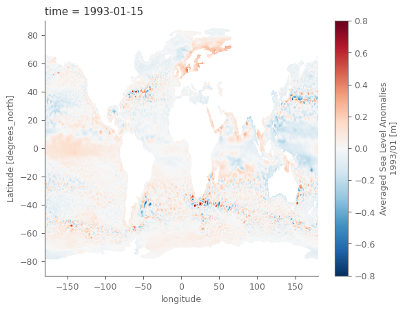
Finally, we will only use the sla variable (sea level anomalies) from the dataset, as this is the variable of interest.
# change longitudes to -180 | 180
sla = sea_level['sla']
sla = sla.assign_coords(longitude=(((sla.longitude + 180) % 360) - 180)) # change longitudes
sla = sla.sortby('longitude') # sort by ascending order
sla
<xarray.DataArray 'sla' (time: 355, latitude: 720, longitude: 1440)>
dask.array<getitem, shape=(355, 720, 1440), dtype=float64, chunksize=(1, 720, 1440), chunktype=numpy.ndarray>
Coordinates:
  * time       (time) datetime64[ns] 1993-01-15 1993-02-15 ... 2022-07-15
  * latitude   (latitude) float32 -89.88 -89.62 -89.38 ... 89.38 89.62 89.88
  * longitude  (longitude) float32 -179.9 -179.6 -179.4 ... 179.4 179.6 179.9
Attributes:
    cell_methods:   time: mean within years
    grid_mapping:   crs
    long_name:      Averaged Sea Level Anomalies 1993/01
    standard_name:  sea_surface_height_above_sea_level
units: m# "quick and dirty" plot of the data
sla.isel(time=0).plot()
<matplotlib.collections.QuadMesh at 0x7ff0e1160220>
Section 3. Data analysis and plotting#
Global average#
The data are projected in lat/lon system. This system does not have equal areas for all grid cells, but as we move closer to the poles, the areas of the cells are reducing. These differences can be accounted when weighting the cells with the cosine of their latitude.
def area_weighted_spatial_average(data):
    """Calculate area-weighted spatial average of data

    Parameters
    ----------
    data : xarray.DataArray
        DataArray with lat and lon coordinates

    Returns
    -------
    xarray.DataArray
        Area-weighted spatial average

    """
    weights = np.cos(np.deg2rad(data.latitude)).clip(0, 1) # weights; clip ensures values are between 0 and 1
    return data.weighted(weights).mean(['latitude', 'longitude'])
Calculate global average sea level anomaly for the monthly timeseries. This will take a while…
global_average_sla = area_weighted_spatial_average(sla).compute() # use compute so that the data are now loaded into memory (no more dask)
# quick plot
global_average_sla.plot(figsize=(4, 2))
[<matplotlib.lines.Line2D at 0x7ff0e202a5f0>]
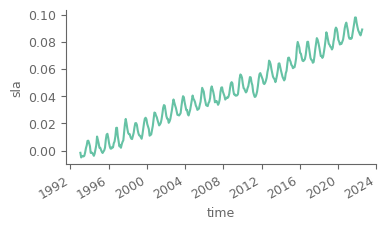
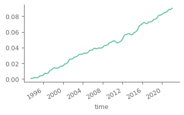
Notice that there is a high seasonal fluctuation in the dataset. Let’s use a low-pass filter considering a 13-month (6 months before/after) moving average for mitigating the effect of seasonality. As the data are monthly and each month has different number of days, we will use weigths for an accurate representation of the smoothing.
smoothed_n_months = 13 # months used for the temporal smoothing

# get number of days for each month
years = global_average_sla.time.dt.year.values
months = global_average_sla.time.dt.month.values
days_month = [calendar.monthrange(yr, mn)[1] for yr, mn in zip(years, months)]

# temporal weights as xarray object (helps with automated alignment of the data for the calculations at the next steps)
weights_temporal = global_average_sla.time.astype(int)*0+days_month

# weights should be changed to NaN for the cells that hava NaN in the relevant month
weights_temporal = weights_temporal.where(global_average_sla.notnull())

# rolling sum of the product of satellite measurements with the days per month
temp_smoothed = (global_average_sla*weights_temporal).rolling(time=smoothed_n_months, min_periods=smoothed_n_months, center=True).sum()

# divide with total number of days for getting the final weighted temporally-smoothed timeseries
temp_smoothed = temp_smoothed/weights_temporal.rolling(time=smoothed_n_months, min_periods=smoothed_n_months, center=True).sum()
temp_smoothed.plot(figsize=(4, 2))
[<matplotlib.lines.Line2D at 0x7ff0e19e5ae0>]
Annual trend calculation#
Let’s calculate the annual trend for the data. For this step, first we will resample the monthly data to annual so that we don’t have influence of possible variations of higher frequency, as for example the seasonality.
Resample the monthly data to annual by weighting the months considering the total number of days per month.
def annual_weighted_mean(data):
    """Calculate weighted annual mean from monthly data, when considering the exact number of days for each month for getting the weights

    Parameters
    ----------
    data : xarray.DataArray
        DataArray with time coordinates in monthly resolution

    Returns
    -------
    xarray.DataArray
        Weighted annual mean

    """

    annual_mean = []
    for i, j in data.groupby('time.year'): # group data per year
        days_month = [calendar.monthrange(yr, mn)[1] for yr, mn in zip([i]*len(j.time), j.time.dt.month.values)] # get number of days per month
        # weights should be changed to NaN for the cells that have NaN in the relevant month
        weights_temporal = j.time.astype(int)*0+days_month # get the weights
        weights_temporal = weights_temporal.where(j.notnull()).fillna(0) # mask weights for all instances with no data, and get weights to 0

        annual_mean.append( j.weighted(weights_temporal).mean('time').assign_coords(year=i) ) # get the weighted mean

    annual_mean = xr.concat(annual_mean, dim='year') # get final dataarray with the annual growth rates

    return annual_mean
Calculate global average sea level anomaly for the annual data.
global_average_annual_sla = annual_weighted_mean(global_average_sla)

# be presice with the time and assign the middle of each year. For the last year adjust based on the last month available on the raw data
full_years = global_average_annual_sla.year[:-1].values+.5
last_year = global_average_annual_sla.year[-1].values+global_average_sla.time[-1].dt.month.values/12*.5
new_year_coords = np.append(full_years, last_year)
global_average_annual_sla = global_average_annual_sla.assign_coords({'year': new_year_coords})

global_average_annual_sla.to_dataset() # we use 'dataset' object instead of 'dataarray' so that the information are visually nicer
<xarray.Dataset>
Dimensions:  (year: 30)
Coordinates:
  * year     (year) float64 1.994e+03 1.994e+03 ... 2.022e+03 2.022e+03
Data variables:
sla (year) float64 0.0002212 0.00159 0.003856 ... 0.08853 0.08751Use linregress from the scipy library and appply_func from the xarray library for calculating the linear trend and the standard error of the estimated slope. More information are available in the documentations of scipy and xarray. Let’s also split the data in first and second half to understand if there are variations in the trends.
def linregress_1d(data, years):

    """
    The function returns an array with 5 elements. The 1st and 2nd element are the slope and intersect of the regression, and the 5th value
    is the standard error of the estimated slope.
    """

    return np.array(linregress(years, data)[:])
period_of_interest = {
    'Full': {'year': slice(1993, 2022)},
    'Half1': {'year': slice(1993, 2007)},
    'Half2': {'year': slice(2008, 2022)},
}
global_trend = []
for name, period in period_of_interest.items():
    data = global_average_annual_sla.sel(period) # select the period of interest
    trend = xr.apply_ufunc(linregress_1d,
                           data*1e3, data.year.values, # get the data from m to mm
                           input_core_dims=[["year"], ['t']], output_core_dims=['a'], vectorize=True) # get 1st order linear trend
    trend = trend.assign_coords({'period': name}) # add new coordinate so that we can later on contatenate the data in one dataarray object
    global_trend.append(trend) # append the xarray object to the list

global_trend = xr.concat(global_trend, dim='period') # concat the xarray objests of the list, into 1 single xarray dataarray
global_trend.isel(a=0) # check the slops (1st element)
<xarray.DataArray 'sla' (period: 3)>
array([3.10341283, 3.15749711, 3.63171855])
Coordinates:
  * period   (period) <U5 'Full' 'Half1' 'Half2'
There is a slight differentiation on the linear trend, with the 2nd half having a steeper increase.
Caclulate fitted values for the linear trend.
time_float = global_average_sla.time.dt.year + global_average_sla.time.dt.dayofyear/365 # get monthly time as float
linear_fit = global_trend.sel(period='Full')[0]*time_float + global_trend.sel(period='Full')[1] # get fitted timeseries based on linear trend
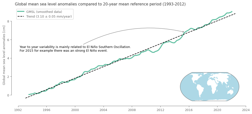
Plotting the monthly timeseries#
fig, ax = plt.subplots(1, 1, figsize=(12, 5)) # create the figure and define subplots and figure size

p1 = (100*temp_smoothed).plot(ax=ax, linewidth=3) # plot in cm rather than m that is the unit of the data
p2 = (.1*linear_fit).plot(ax=ax, linestyle='--', color='black') # plot the trend data (need to convert to cm from mm)

# add legend
ax.legend([p1[0], p2[0]],
          ['GMSL (smoothed data)',
          f"Trend ({global_trend.sel(period='Full')[0]:0.2f} \u00B1 {global_trend.sel(period='Full')[4]:0.2f} mm/year)"],
          loc=2)

# formatting the figure
sns.despine(ax=ax, trim=True, offset=10) # trimming the y and x axis to be visible only from the first till the last tick
ax.xaxis.set_major_formatter(mdates.DateFormatter('%Y')) # formatting is needed cause the above line breaks the time xticklabels

ax.set_xlabel('') # remove the title from the horizontal axis
ax.set_ylabel('Global mean sea level anomalies [cm]') # set title in vertical axis
ax.set_title('Global mean sea level anomalies compared to 20-year mean reference period (1993-2012)') # set title for the subplot

# add a small map showing the spatial domain that was used to derive the timeseries. This will be done with the help of inset_axes
axins = inset_axes(ax, # define the parent subplot
                   width="30%", height="30%", loc="lower right", # give dimensions and location of the nested subplot
                   axes_class=cartopy.mpl.geoaxes.GeoAxes, # define subplot class so that geospatial data can be used
                   axes_kwargs=dict(projection=ccrs.EqualEarth()) # assign a projection in the nested subplot
                   )
axins.add_feature(cfeature.OCEAN, color='lightblue', lw=.5) # add the oceans as polygons from the cartopy library

# add text regarding the increase of sea level in 2015
desc = 'Year to year variability is mainly related to El Niño Southern Oscillation.\nFor 2015 for example there was an strong El Niño event.'
ax.annotate(
               desc,
               xy=(pd.to_datetime('20150615'), temp_smoothed.sel(time=pd.to_datetime('20150615'))*100),
               xytext=(0.02, 0.6),
               color='black',
               textcoords=ax.transAxes,
               ha='left', va='top',
               arrowprops=dict(arrowstyle='->', color='grey', connectionstyle='arc3,rad=-0.2')
            )

plt.show()
Variations in space#
We noticed that there is an increasing trend in the global average sea level. Let’s now calculate this trend for each grid point using the same simple linear model we used previously.
First of all we need to rechunk the data so that the time dimension is not segmented, because the trend calculation needs all time steps for each location.
sla = sla.chunk(chunks={'time': -1, 'latitude': 72, 'longitude': 144}) # rechunk so time is not segmented (needed for trends)
sla
<xarray.DataArray 'sla' (time: 355, latitude: 720, longitude: 1440)>
dask.array<rechunk-merge, shape=(355, 720, 1440), dtype=float64, chunksize=(355, 72, 144), chunktype=numpy.ndarray>
Coordinates:
  * time       (time) datetime64[ns] 1993-01-15 1993-02-15 ... 2022-07-15
  * latitude   (latitude) float32 -89.88 -89.62 -89.38 ... 89.38 89.62 89.88
  * longitude  (longitude) float32 -179.9 -179.6 -179.4 ... 179.4 179.6 179.9
Attributes:
    cell_methods:   time: mean within years
    grid_mapping:   crs
    long_name:      Averaged Sea Level Anomalies 1993/01
    standard_name:  sea_surface_height_above_sea_level
units: mCalculate mean annual anomalies of sea level. This will take a while…
average_annual_sla = annual_weighted_mean(sla).compute() # once again we use compute so that the calculated data are stored in the memory
average_annual_sla.to_dataset() # remember that we use 'dataset' object instead of 'dataarray' so that the information are visually nicer
<xarray.Dataset>
Dimensions:    (latitude: 720, longitude: 1440, year: 30)
Coordinates:
  * latitude   (latitude) float32 -89.88 -89.62 -89.38 ... 89.38 89.62 89.88
  * longitude  (longitude) float32 -179.9 -179.6 -179.4 ... 179.4 179.6 179.9
  * year       (year) int64 1993 1994 1995 1996 1997 ... 2019 2020 2021 2022
Data variables:
sla (year, latitude, longitude) float64 nan nan nan ... nan nan nanCalculate the annual trend, again with the help of apply_func.
gridded_trend = xr.apply_ufunc(linregress_1d,
                               average_annual_sla*1e3, average_annual_sla.year.values,
                               input_core_dims=[["year"], ['t']], output_core_dims=['a'], vectorize=True)
gridded_trend.to_dataset() # remember that we use 'dataset' object instead of 'dataarray' so that the information are visually nicer
<xarray.Dataset>
Dimensions:    (latitude: 720, longitude: 1440, a: 5)
Coordinates:
  * latitude   (latitude) float32 -89.88 -89.62 -89.38 ... 89.38 89.62 89.88
  * longitude  (longitude) float32 -179.9 -179.6 -179.4 ... 179.4 179.6 179.9
Dimensions without coordinates: a
Data variables:
sla (latitude, longitude, a) float64 nan nan nan nan ... nan nan nantrends_slope = gridded_trend.isel(a=0) # get the slice with the slope data (remember it is the 1st value)
Plotting gridded data#
def spatial_plot(data_used, projection_used, figsize):

    # get colors and levels for the plotting
    levels = np.linspace(-6, 6, 25)
    colormap = sns.color_palette('GnBu_r', n_colors=13) + sns.color_palette('YlOrRd', n_colors=13)
    colormap = ListedColormap(colormap)

    # plot the data
    fig, ax = plt.subplots(1, 1, figsize=figsize, subplot_kw={'projection': projection_used}) # create the figure and ax

    slope_plot = data_used.plot(vmin=-6, vmax=6, cmap=colormap, levels=levels, extend='both', # plot the gridded data
                                add_colorbar=False, robust=True, ax=ax, transform=ccrs.PlateCarree())

    ax.add_feature(cfeature.NaturalEarthFeature(category='physical', scale='10m', facecolor='0', name='land')) # add land mask

    # add colorbar and plot inside it the boxplot of the trends ( only for the values within [-6, 6] ), for visualizing also the statistics
    cbar_ax = fig.colorbar(slope_plot, extend='both', label='mm/year') # add colorbar
    cbar_ax.ax.boxplot(x=data_used.to_dataframe().dropna().values, # boxplot of the trend data
                       positions=[.5], # define position at 0.5 so that the data are plotted in the middle of colorbar (0-1), because default is 1
                       widths=0.5, # slightly increase the width of the boxplot
                       patch_artist=True, # allow changes on the boxplot
                       showmeans=True, # also show the mean
                       boxprops=dict(facecolor='.8'), # change color of boxplot (so that median is more visible)
                       medianprops=dict(color='black'),
                       flierprops={'marker': '+', 'markersize': 2}, # change style and size of outliers
                       meanprops={'markerfacecolor': 'white', 'markeredgecolor': 'black', 'marker': 'o'} # change of mean symbol
                       )
    cbar_ax.ax.set_xticks([]) # remove the xticks due to the boxplot from the colorbar

    return fig, ax
fig, ax = spatial_plot(data_used=trends_slope.sel(latitude=slice(24, 83), longitude=slice(-30, 55)), projection_used=ccrs.PlateCarree(), figsize=(11, 6))

# add title with the location and the years used for calculating the trend
min_year, max_year = average_annual_sla.year.values[::len(average_annual_sla.year)-1] # get min and max year of data
ax.set_title(f'Sea level trends from satellite altimetry in European seas from {min_year} to {max_year}')

plt.show()
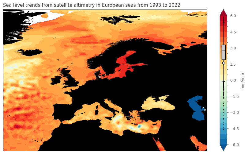
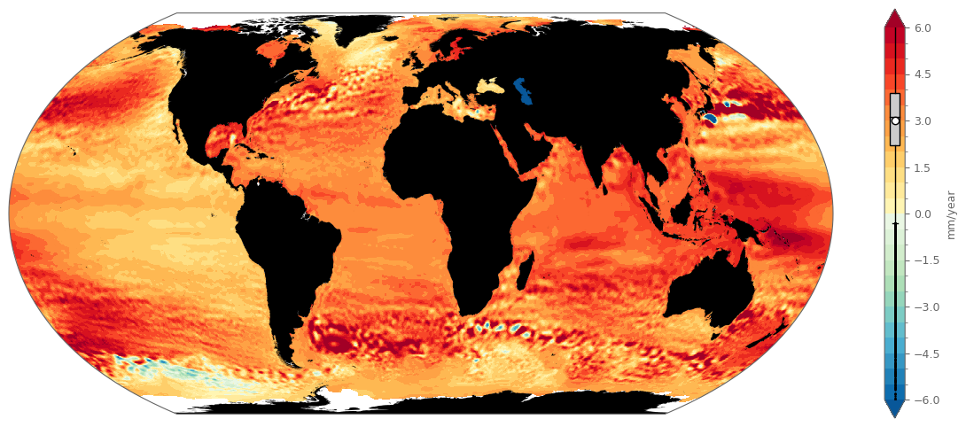
The above plot shows that for the majority of the European seas there is an increasing trend in the sea level, ranging between 2-3 mm/year, whereas some regions experience an increase over 5 mm/year. Decreasing trends are very rare, mainly in confined parts of east Mediterraean (south of Creta island and in the Ionian sea, between mainland Greece and Italy).
Please note that the Caspian Sea has a substantial descrease, but this is not related to the sea level, as it is a closed system (lake) that is not affected by changes in the sea ice in the poles. This decrease is rather related to the increasing temperature and higher evaporation, as well as intensive human activities.
SUMMARY:
In this tutorial we analysed the changes in sea level anomalies.
The data showed that the sea level is constantly inceasing the last years, with a trend over 3mm/year for the global average. Looking at the seas sourounding Europe, there is an overal increasing trend with a strong spatial variability. The regions in the Baltic have some of the most increasing trends (over 5mm/year), while locations in the east Mediterraean have a smaller slope, with even decreasing trends for some parts of the area.
Appendix#
NOTE:
The plots in the relevant Climate Indicators Report are created after a detailed preprocessing of the data for correcting known issues and caclulating the uncertainty in the trends. Such a detailed processing is not in the scope of this tutorial. Nevertheless, for the interested users, this appendix consists of two sections that present some additional datasets that can be used for this analysis. More specifically:
The 1st section contains processed data downloaded from the Copernicus Marine Service.
The 2nd section contains a brief demonstration of how to use the daily data of sea level anomalies from CDS. Remember that this analysis requires a lot of time for downloading the data (more than half a day in most cases), and over 90 Gb of space on the disk.
Section 1: Processed data from Marine Service.#
For getting data from Marine Service, there is a free user registration needed. The data can then be downloaded from an ftp server.
marine_username = '########' # please add your username
marine_password = '########' # please add your password
Download the already processed area weighted mean sea level anomaly timeseries.#
# define the url for getting the data and add the username and password
marine_sla_timeseries = f"ftp://{marine_username}:{marine_password}@my.cmems-du.eu/Core/GLOBAL_OMI_SL_area_averaged_anomalies/"
marine_sla_timeseries += "global_omi_sl_area_averaged_anomalies/global_omi_sl_area_averaged_anomalies_19930101_P20230403.nc"

urllib.request.urlretrieve(marine_sla_timeseries, f'{dir_loc}timeseries_marine.nc') # retrieve the data and store them in the directory
marine_sla_timeseries = xr.open_dataset(f'{dir_loc}timeseries_marine.nc') # read the data
marine_sla_timeseries # view dataset
<xarray.Dataset>
Dimensions:               (time: 10808)
Coordinates:
  * time                  (time) datetime64[ns] 1993-01-01 ... 2022-08-04
Data variables:
    sla                   (time) float32 ...
    sla_filtered          (time) float32 ...
    sla_tpacorr           (time) float32 ...
    sla_filtered_tpacorr  (time) float32 ...
Attributes:
    title:        Area Averaged Mean Sea Level from DUACS DT2021
    institution:  CLS
    references:   http://marine.copernicus.eu
    Conventions:  CF-1.7
    source:       The values are based on the two-satellite merged altimeter ...
    licence:      http://marine.copernicus.eu/services-portfolio/service-comm...
    area:         GLOBAL
    comment:      Period : 1993-01-01 to 2022-08-04.
    credit:       E.U. Copernicus Marine Service Information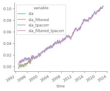
contact: https://marine.copernicus.eu/contactAs we can see from the above cell, the data refer to sea level anomalies (sla) for the period 1st January 1993 - 4th August 2022. There are 4 variables:
sla, which is the original timeseries of area averaged mean seal level
sla_filtered, which has a low-pass filter on the above variable
sla_tpa_corr, which is the original timeseries, after correcting for the TOPEX-A instrumental drift
sla_filtered_tpacorr, low-ass filtered of the above variable
marine_sla_timeseries.to_array().plot(hue='variable', figsize=(4, 3))
plt.show()
Let’s compare the processed daily data from Marine Service with the smoothed timeseries we calculated from the monthly data.
fig, ax = plt.subplots(1, 1, figsize=(12, 5)) # create the figure and define subplots and figure size

marine_sla_timeseries.to_array().plot(hue='variable', ax=ax)
temp_smoothed.plot(ax=ax, linewidth=3, color='black')
plt.show()
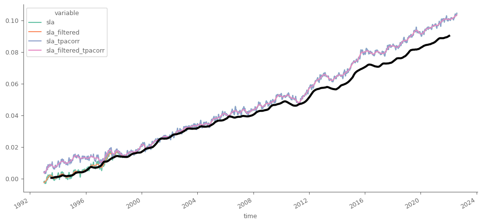
Our calculations have a considerable underestimation of the trend in the second half, as we see that after the preprocessing and the corrections implemented in the data from Marine Copernicus, sea level anomalies are substantially higher for the processed data for the last years. The main reason is the incorporation of the glacial rebound on the processed data from Marine Service. We will conduct this processing at the Section 2 of this Appendix.
Download the trends of sea level.#
marine_sla_trends = f"ftp://{marine_username}:{marine_password}@my.cmems-du.eu/Core/GLOBAL_OMI_SL_regional_trends/"
marine_sla_trends += "global_omi_sl_regional_trends/global_omi_sl_regional_trends_19930101_P20230403.nc"

urllib.request.urlretrieve(marine_sla_trends, f'{dir_loc}trends_marine.nc')
marine_sla_trends = xr.open_dataset(f'{dir_loc}trends_marine.nc')
marine_sla_trends
<xarray.Dataset>
Dimensions:    (latitude: 720, longitude: 1440)
Coordinates:
  * latitude   (latitude) float32 -89.88 -89.62 -89.38 ... 89.38 89.62 89.88
  * longitude  (longitude) float32 -179.9 -179.6 -179.4 ... 179.4 179.6 179.9
Data variables:
    msl_trend  (latitude, longitude) float32 ...
Attributes:
    title:                         Merged gridded regional mean sea level tre...
    institution:                   CLS
    references:                    http://marine.copernicus.eu
    Conventions:                   CF-1.7
    source:                        The values are based on the two-satellite ...
    licence:                       http://marine.copernicus.eu/services-portf...
    quality_information_document:  http://marine.copernicus.eu/documents/QUID...
    product_user_manual:           http://marine.copernicus.eu/documents/PUM/...
    area:                          GLOBAL
    comment:                       Period : 1993-01-01 to 2022-08-04.
    credit:                        E.U. Copernicus Marine Service Information
contact: https://marine.copernicus.eu/contactGenerate same plot as the monthy data from CDS.
fig, ax = spatial_plot(data_used=marine_sla_trends['msl_trend'].sel(latitude=slice(24, 83), longitude=slice(-30, 55)),
                       projection_used=ccrs.PlateCarree(), figsize=(11, 6))

# add title with the location and the years used for calculating the trend
min_year, max_year = marine_sla_timeseries.time.dt.year.values[::len(marine_sla_timeseries.time.dt.year)-1] # get min and max year of data
ax.set_title(f'Sea level trends from satellite altimetry in European seas from {min_year} to {max_year} - Marine Copernicus')

plt.show()
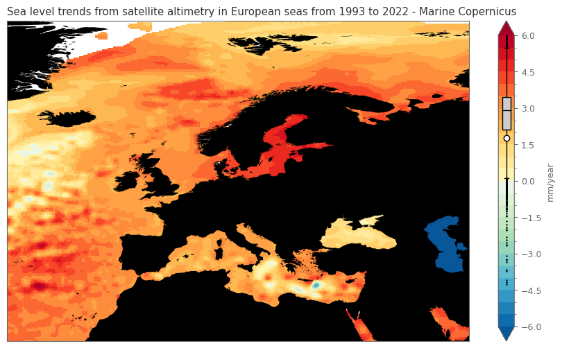
The trends in Europe with the processed data from Marine Service are highly resembling the calculated trends from the monthly data. This could be related to the fact that the spatial data in the Climate Indicator Report are not undercome extensive processing for corrections, as the case with the global average timeseries.
fig, ax = spatial_plot(data_used=marine_sla_trends['msl_trend'], projection_used=ccrs.EqualEarth(), figsize=(15, 6))
Section 2: Get daily data from CDS.#
This requires ~100Gb of data and a considerable amount of time (~1 day order of magnitude) for downloading the data and performing the calculations…
os.makedirs(f'{dir_loc}/daily/', exist_ok=True) # create the folder if not available
c = cdsapi.Client(url=cds_url, key=cds_key)

# we need to loop every year, otherwise the data are too many to be downloaded from CDS
# for i_year in range(1993, 2023):
for i_year in range(1993, 1995): # use only 2 years just for speeding up the process and reducing the time (it still needs some hours)
    c.retrieve(
        'satellite-sea-level-global',
        {
            'version': 'vDT2021',
            'format': 'zip',
            'variable': 'daily',
            'year': i_year,
            'month': [('0'+str(i))[-2:] for i in list(range(1, 13))], # the months should be given as 2digit (e.g., '01', '12'),
            'day': [('0'+str(i))[-2:] for i in list(range(1, 32))], # the days should be given as 2digit (e.g., '01', '31'),
        },
        f'{dir_loc}/daily/{i_year}_sea_level.zip')

    # unzip and remove the original file
    with zipfile.ZipFile(f'{dir_loc}/daily/{i_year}_sea_level.zip','r') as zip_ref:
        zip_ref.extractall(f'{dir_loc}/daily/') # unzip file

    os.remove(f'{dir_loc}/daily/{i_year}_sea_level.zip') # delete the original zip file
Find all month-years that there are available files. The idea is to read the files per month-year so that we don’t load lot of data in memory. We could in fact read all files at once, since dask can handle the size. This will nevertheless substantially increase the computation time.
all_yearmonths = list(set([i.split('_')[5][:-2] for i in os.listdir(f'{dir_loc}/daily/')]))
all_yearmonths = list(sorted(all_yearmonths))
Let’s now create a function for reading all files for the month-year and calculate global average at a daily resolution, as well as monthly average for each grid cell.
def data_processing(yearmonth):

    # first read all files of the relevant yearmonth
    data = xr.open_mfdataset(f'{dir_loc}/daily/dt_global_twosat_phy_l4_{yearmonth}*.nc').load() # load on memory (year-month data have manageable size)

    # calculate global weighted average
    global_average = area_weighted_spatial_average(data)
    global_average.to_netcdf(f'{dir_loc}/processed/global_average_daily_{yearmonth}.nc')

    # # calculate monthly average
    # data_monthly = data.mean('time')
    # data_monthly = data_monthly.assign_coords({'time': yearmonth}).expand_dims('time')

    # data_monthly.to_netcdf(f'{dir_loc}/processed/data_monthly_{yearmonth}.nc') # requires a lot more storage than 1 sinle daily file; need further investigation
    # for the above check https://stackoverflow.com/questions/72112551/significant-increase-in-file-size-x10-after-applying-function-on-netcdf-data-u

    # return data_monthly
The below cell needs around 6 hours to complete if all data (from year 1993 to year 2022) are donwloaded.
from tqdm import tqdm
os.makedirs(f'{dir_loc}/processed/', exist_ok=True) # create the folder if not available
for i_yearmonth in tqdm(all_yearmonths):
    data_processing(i_yearmonth)
global_ts_daily = xr.open_mfdataset(f'{dir_loc}/processed/*.nc')
global_ts_daily = global_ts_daily.sortby('time').load()
global_ts_daily.to_netcdf(f'{dir_loc}/timeseries_daily.nc')
global_ts_daily = xr.open_dataset(f'{dir_loc}/timeseries_daily.nc')
global_ts_daily
<xarray.Dataset>
Dimensions:         (time: 10808, nv: 2)
Coordinates:
  * time            (time) datetime64[ns] 1993-01-01 1993-01-02 ... 2022-08-04
  * nv              (nv) int32 0 1
Data variables: (12/14)
    crs             (time) float64 ...
    lat_bnds        (time, nv) float32 ...
    lon_bnds        (time, nv) float32 ...
    sla             (time) float64 ...
    err_sla         (time) float64 ...
    ugosa           (time) float64 ...
    ...              ...
    err_vgosa       (time) float64 ...
    adt             (time) float64 ...
    ugos            (time) float64 ...
    vgos            (time) float64 ...
    tpa_correction  (time) float64 ...
flag_ice (time) float64 ...Let’s process our daily timeseries with the below two steps:
remove the seasonal cycle
adjust for the post-glacial rebound, considering an increase of 0.3 mm/year for the global mean sea level trend (more information at Spada, 2016, and Peltier, 2004)
# Step 1: remove seasonal cycle
global_ts_daily_processed = global_ts_daily['sla'].groupby('time.month') - global_ts_daily['sla'].groupby('time.month').mean() # remove monthly climatology
global_ts_daily_processed = global_ts_daily_processed + global_ts_daily['sla'].mean() # add the mean state, so that we don't have anomalies, as in the previous line


# Step 2: adjust for the post-glacial rebound
post_glacial_rebound = global_ts_daily_processed.resample(time='Y').mean()*0 # new dataframe of yearly resolution filled with 0 everywhere
post_glacial_rebound += (np.arange(0, len(post_glacial_rebound))*0.3)/1000 # add 0.3 mm/year trend, but use m as umits
post_glacial_rebound = post_glacial_rebound.resample(time='d').mean().interpolate_na(dim='time', method='linear') # convert back to daily and proportioanlly split the yearly trend
post_glacial_rebound = post_glacial_rebound.isel(time=range(1, len(post_glacial_rebound.time))) # don't use the first day (last day of 1993, because it will be added at the next step)
post_glacial_rebound = xr.concat([global_ts_daily_processed.sel(time='1993').drop('month')*0, post_glacial_rebound], dim='time') # add all days of the first year; this year has no adjustment

# Final processed timeseries
global_ts_daily_final = global_ts_daily_processed + post_glacial_rebound
marine_sla_timeseries['sla'].plot(color='blue', label='Marine', linewidth=1, alpha=.7, figsize=(14, 7)) # plot data from Marine Service
global_ts_daily_final.plot(color='red', label='CDS daily', linewidth=1, alpha=.7) # plot processed daily data
global_ts_daily_final.rolling(time=15, min_periods=1, center=True).mean().plot(color='black', label='CDS daily smoothed', linewidth=1, alpha=.7) # smoothed
plt.legend()
plt.show()
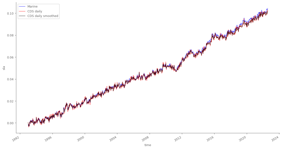
We see that the available (already processed) data from Marine serive, and the data we processed from the daily CDS files are very very similar. Small differences are related to the extra processing steps done by Marine service, as for example removing the semi-annual period signal.