Chapter 6: Climate Oscillations

This chapter delves into two of the most renowned climate oscillations: the El Niño-Southern Oscillation (ENSO) and the North Atlantic Oscillation (NAO). ENSO is an ocean-atmosphere oscillation in the tropical Pacific Ocean with a period spanning 2-7 years, while the NAO operates in the North Atlantic Ocean over a period of 5-10 years. Both these oscillations considerably influence the climate of nearby continents. In this chapter, we’ll investigate how to formulate indices that represent the state of these climate oscillations. Additionally, we’ll briefly delve into how one might identify teleconnections, using surface temperature teleconnections of ENSO as an illustrative example.

Objective:
Craft indices for ENSO and NAO climate oscillations analogous to Figure 5 in Climate Indicators/Sea Surface Temperature and Figure 3 in ESOTC 2022/Atmospheric Circulation. Afterwards, explore the teleconnections of ENSO.

Caution:
This notebook is notably data-heavy and necessitates roughly 20 GB of free disk space. Cells in the notebook that initiate a download will be preceded by a warning cell.

NOTE: Before interacting with the following notebook, please ensure you've reviewed the How to Execute the Notebooks section.

Run the tutorial via free cloud platforms:

---

Importing Packages

Begin by importing the requisite packages for this tutorial.

# API and system utilities
import cdsapi
import os

# Data manipulation and computation
import xarray as xr
import numpy as np
import dask
import datetime as dt

# Data visualization and plotting
import matplotlib.pyplot as plt
import matplotlib.dates as dates
import matplotlib.ticker as ticker
import seaborn as sns
import cartopy.crs as ccrs
import cartopy.feature as cfeature

# EOF analysis
import xeofs as xe

# Progress bars and diagnostics
from tqdm.notebook import tqdm
from dask.diagnostics import ProgressBar

Execute the cell below to adopt this book’s visualisation style. This ensures consistency in visual presentations throughout the notebook. Note, this solely pertains to visualisation and doesn’t affect the underlying calculations. If using GoogleColab, the matplotlib stylesheet won’t be unavailable.

plt.style.use("../copernicus.mplstyle")

To optimise dask’s performance, avoid generating large dask chunks.

dask.config.set(**{'array.slicing.split_large_chunks': True})

<dask.config.set at 0x7fee6c2aba00>

Getting Started

Establish the reference period which characterises the climatology of our datasets.

REF_PERIOD = dict(time=slice('1991', '2020'))

We’ll also define a set of projections for cartopy to be used subsequently.

proj = {
    "data": ccrs.PlateCarree(),
    "map_global": ccrs.Robinson(central_longitude=180),
    "map_north_atlantic": ccrs.Orthographic(central_longitude=-20, central_latitude=60),
}

Moving forward, set up a data directory to neatly store our files.

path_to = {}  # dictionary containing [<variable> : <target folder>]

path_to.update({"temp": "data/temp/era5_temp.nc"})
path_to.update({"temp_anomalies": "data/temp/era5_temp_anomalies.nc"})
path_to.update({"gph": "data/gph/era5_gph.nc"})

for file, path in path_to.items():
    os.makedirs(os.path.dirname(path), exist_ok=True)
    print("{:<20} --> {}".format(file, path))

temp                 --> data/temp/era5_temp.nc
temp_anomalies       --> data/temp/era5_temp_anomalies.nc
gph                  --> data/gph/era5_gph.nc

ENSO Index

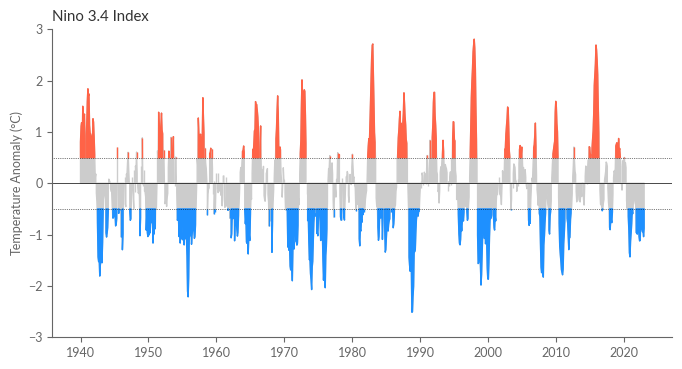
Our first step is to derive the ENSO index using sea surface temperature (SST) data from the ERA5 reanalysis. While there are multiple methods to derive the ENSO index, our approach utilises the NINO3.4 index. This index denotes the average SST anomalies within the region 5°S-5°N, 170°W-120°W.

Downloading Data

Kick off by downloading the data from the Climate Data Store (CDS). We’re particularly interested in the monthly averaged SST data from ERA5 reanalysis. The CDS API is our tool of choice for this download. Given that the NINO3.4 index is constrained to a specific spatial region, one might consider downloading only this section. Yet, since our aim is to later probe the surface temperature teleconnections of ENSO, we’ll encompass global data. This includes downloading the monthly averaged 2m temperature data from ERA5 reanalysis. Enter your CDS API key in the cell below.

New to CDS? Consider the CDS tutorial for a detailed guide.

Please input your CDS API key in the subsequent cell.

##### ERA5 reanalysis
URL = 'https://cds.climate.copernicus.eu/api/v2'
KEY = '##################################' # add your key here the format should be as {uid}:{api-key}

Now, let’s initiate the data download.

Warning:
The upcoming cell will download approximately 4 GB. Ensure you have sufficient storage space. Depending on your internet speed, this could take several hours.

c = cdsapi.Client(url=URL, key=KEY)

c.retrieve(
  'reanalysis-era5-single-levels-monthly-means',
  {
    'format': 'netcdf',
    'product_type': 'monthly_averaged_reanalysis',
    'variable': ['2m_temperature', 'sea_surface_temperature'],
    'year': list(range(1940, 2023)),
    'month': list(range(1, 13)),
    'time': '00:00',
  },
  path_to['temp']
)

We’ll then lazily load the data employing xarray and dask. Our chunks will be set by spatial dimensions rather than time, considering our calculations will operate along the time axis.

temperatures = xr.open_mfdataset(path_to["temp"], chunks={"time": -1, "longitude": 300, "latitude": 150})
temperatures

<xarray.Dataset>
Dimensions:    (longitude: 1440, latitude: 721, time: 996)
Coordinates:
  * longitude  (longitude) float32 0.0 0.25 0.5 0.75 ... 359.0 359.2 359.5 359.8
  * latitude   (latitude) float32 90.0 89.75 89.5 89.25 ... -89.5 -89.75 -90.0
  * time       (time) datetime64[ns] 1940-01-01 1940-02-01 ... 2022-12-01
Data variables:
    t2m        (time, latitude, longitude) float32 dask.array<chunksize=(996, 150, 300), meta=np.ndarray>
    sst        (time, latitude, longitude) float32 dask.array<chunksize=(996, 150, 300), meta=np.ndarray>
Attributes:
    Conventions:  CF-1.6
    history:      2023-09-11 17:33:49 GMT by grib_to_netcdf-2.25.1: /opt/ecmw...

xarray.Dataset

• Dimensions:
  • longitude: 1440
  • latitude: 721
  • time: 996
• Coordinates: (3)
  • longitude
    (longitude)
    float32
    0.0 0.25 0.5 ... 359.2 359.5 359.8

    units :

    degrees_east

    long_name :

    longitude

    array([0.0000e+00, 2.5000e-01, 5.0000e-01, ..., 3.5925e+02, 3.5950e+02,
           3.5975e+02], dtype=float32)

  • latitude
    (latitude)
    float32
    90.0 89.75 89.5 ... -89.75 -90.0

    units :

    degrees_north

    long_name :

    latitude

    array([ 90.  ,  89.75,  89.5 , ..., -89.5 , -89.75, -90.  ], dtype=float32)

  • time
    (time)
    datetime64[ns]
    1940-01-01 ... 2022-12-01

    long_name :

    time

    array(['1940-01-01T00:00:00.000000000', '1940-02-01T00:00:00.000000000',
           '1940-03-01T00:00:00.000000000', ..., '2022-10-01T00:00:00.000000000',
           '2022-11-01T00:00:00.000000000', '2022-12-01T00:00:00.000000000'],
          dtype='datetime64[ns]')

• Data variables: (2)
  • t2m
    (time, latitude, longitude)
    float32
    dask.array<chunksize=(996, 150, 300), meta=np.ndarray>

    units :

    K

    long_name :

    2 metre temperature

    Array Chunk Bytes 3.85 GiB 170.97 MiB Shape (996, 721, 1440) (996, 150, 300) Dask graph 25 chunks in 2 graph layers Data type float32 numpy.ndarray

  • sst
    (time, latitude, longitude)
    float32
    dask.array<chunksize=(996, 150, 300), meta=np.ndarray>

    units :

    K

    long_name :

    Sea surface temperature

    Array Chunk Bytes 3.85 GiB 170.97 MiB Shape (996, 721, 1440) (996, 150, 300) Dask graph 25 chunks in 2 graph layers Data type float32 numpy.ndarray

• Indexes: (3)
  • longitude
    PandasIndex

    PandasIndex(Float64Index([   0.0,   0.25,    0.5,   0.75,    1.0,   1.25,    1.5,   1.75,
                     2.0,   2.25,
                  ...
                   357.5, 357.75,  358.0, 358.25,  358.5, 358.75,  359.0, 359.25,
                   359.5, 359.75],
                 dtype='float64', name='longitude', length=1440))

  • latitude
    PandasIndex

    PandasIndex(Float64Index([  90.0,  89.75,   89.5,  89.25,   89.0,  88.75,   88.5,  88.25,
                    88.0,  87.75,
                  ...
                  -87.75,  -88.0, -88.25,  -88.5, -88.75,  -89.0, -89.25,  -89.5,
                  -89.75,  -90.0],
                 dtype='float64', name='latitude', length=721))

  • time
    PandasIndex

    PandasIndex(DatetimeIndex(['1940-01-01', '1940-02-01', '1940-03-01', '1940-04-01',
                   '1940-05-01', '1940-06-01', '1940-07-01', '1940-08-01',
                   '1940-09-01', '1940-10-01',
                   ...
                   '2022-03-01', '2022-04-01', '2022-05-01', '2022-06-01',
                   '2022-07-01', '2022-08-01', '2022-09-01', '2022-10-01',
                   '2022-11-01', '2022-12-01'],
                  dtype='datetime64[ns]', name='time', length=996, freq=None))

• Attributes: (2)

  Conventions :

  CF-1.6

  history :

  2023-09-11 17:33:49 GMT by grib_to_netcdf-2.25.1: /opt/ecmwf/mars-client/bin/grib_to_netcdf.bin -S param -o /cache/data1/adaptor.mars.internal-1694453533.3826513-9338-5-6738052d-b422-49f6-9953-36ae2d000357.nc /cache/tmp/6738052d-b422-49f6-9953-36ae2d000357-adaptor.mars.internal-1694453168.8143947-9338-9-tmp.grib

For simplicity’s sake, rename the longitude and latitude dimensions to lon and lat, respectively.

temperatures = temperatures.rename({'longitude': 'lon', 'latitude': 'lat'})

Compute Anomalies

Next, ascertain the monthly climatologies for both datasets across each grid cell. These climatologies will be instrumental in computing the anomalies.

climatologies = temperatures.sel(REF_PERIOD).groupby("time.month").mean()

with ProgressBar():
    climatologies = climatologies.compute()

[########################################] | 100% Completed | 24.15 s

The ensuing cell calculates the temperature anomalies.

anomalies = temperatures.groupby("time.month") - climatologies

/home/nrieger/miniconda3/envs/tutorial/lib/python3.10/site-packages/xarray/core/indexing.py:1443: PerformanceWarning: Slicing with an out-of-order index is generating 83 times more chunks
  return self.array[key]

A major advantage of dask is its capacity to sequence operations until our processed dataset snugly fits into our memory. Nevertheless, repeatedly computing the same dask DataArray can be inefficient. To counter this, we’ll compute this intermediary result, archive it on our disk, and then lazily fetch it for additional processing.

with ProgressBar():
    anomalies.to_netcdf(path_to["temp_anomalies"])

[########################################] | 100% Completed | 241.66 s

Now, let’s reload the temperature anomalies:

anomalies = xr.open_dataset(path_to["temp_anomalies"], chunks={"time": -1, "lon": 300, "lat": 150})

For ease, extract the anomalies of the global surface temperature at 2m (t2m) and the sea surface temperature (sst), placing them in distinct variables.

t2m = anomalies['t2m']
sst = anomalies['sst']
sst

<xarray.DataArray 'sst' (time: 996, lat: 721, lon: 1440)>
dask.array<open_dataset-sst, shape=(996, 721, 1440), dtype=float32, chunksize=(996, 150, 300), chunktype=numpy.ndarray>
Coordinates:
  * lon      (lon) float32 0.0 0.25 0.5 0.75 1.0 ... 359.0 359.2 359.5 359.8
  * lat      (lat) float32 90.0 89.75 89.5 89.25 ... -89.25 -89.5 -89.75 -90.0
  * time     (time) datetime64[ns] 1940-01-01 1940-02-01 ... 2022-12-01
    month    (time) int64 dask.array<chunksize=(996,), meta=np.ndarray>

xarray.DataArray

'sst'

• time: 996
• lat: 721
• lon: 1440

• dask.array<chunksize=(996, 150, 300), meta=np.ndarray>

  Array Chunk Bytes 3.85 GiB 170.97 MiB Shape (996, 721, 1440) (996, 150, 300) Dask graph 25 chunks in 2 graph layers Data type float32 numpy.ndarray

• Coordinates: (4)
  • lon
    (lon)
    float32
    0.0 0.25 0.5 ... 359.2 359.5 359.8

    units :

    degrees_east

    long_name :

    longitude

    array([0.0000e+00, 2.5000e-01, 5.0000e-01, ..., 3.5925e+02, 3.5950e+02,
           3.5975e+02], dtype=float32)

  • lat
    (lat)
    float32
    90.0 89.75 89.5 ... -89.75 -90.0

    units :

    degrees_north

    long_name :

    latitude

    array([ 90.  ,  89.75,  89.5 , ..., -89.5 , -89.75, -90.  ], dtype=float32)

  • time
    (time)
    datetime64[ns]
    1940-01-01 ... 2022-12-01

    long_name :

    time

    array(['1940-01-01T00:00:00.000000000', '1940-02-01T00:00:00.000000000',
           '1940-03-01T00:00:00.000000000', ..., '2022-10-01T00:00:00.000000000',
           '2022-11-01T00:00:00.000000000', '2022-12-01T00:00:00.000000000'],
          dtype='datetime64[ns]')

  • month
    (time)
    int64
    dask.array<chunksize=(996,), meta=np.ndarray>

    Array Chunk Bytes 7.78 kiB 7.78 kiB Shape (996,) (996,) Dask graph 1 chunks in 2 graph layers Data type int64 numpy.ndarray

• Indexes: (3)
  • lon
    PandasIndex

    PandasIndex(Float64Index([   0.0,   0.25,    0.5,   0.75,    1.0,   1.25,    1.5,   1.75,
                     2.0,   2.25,
                  ...
                   357.5, 357.75,  358.0, 358.25,  358.5, 358.75,  359.0, 359.25,
                   359.5, 359.75],
                 dtype='float64', name='lon', length=1440))

  • lat
    PandasIndex

    PandasIndex(Float64Index([  90.0,  89.75,   89.5,  89.25,   89.0,  88.75,   88.5,  88.25,
                    88.0,  87.75,
                  ...
                  -87.75,  -88.0, -88.25,  -88.5, -88.75,  -89.0, -89.25,  -89.5,
                  -89.75,  -90.0],
                 dtype='float64', name='lat', length=721))

  • time
    PandasIndex

    PandasIndex(DatetimeIndex(['1940-01-01', '1940-02-01', '1940-03-01', '1940-04-01',
                   '1940-05-01', '1940-06-01', '1940-07-01', '1940-08-01',
                   '1940-09-01', '1940-10-01',
                   ...
                   '2022-03-01', '2022-04-01', '2022-05-01', '2022-06-01',
                   '2022-07-01', '2022-08-01', '2022-09-01', '2022-10-01',
                   '2022-11-01', '2022-12-01'],
                  dtype='datetime64[ns]', name='time', length=996, freq=None))

• Attributes: (0)

Now, computing the NINO3.4 index is straightforward. We simply average the weighted SST anomalies in the region 5°S-5°N, 170°W-120°W. Note that as the longitude dimensions ranges from 0 to 360°E, the region defintion translates to 190°E-240°E.

nino34 = sst.sel(lon=slice(190, 240), lat=slice(5, -5))

As we’ve demonstrated in the previous notebooks, we compute the spatial average by weighting the grid cells by the cosine of their latitude. This is to account for the convergence of the meridians at the poles.

weights = np.cos(np.deg2rad(nino34.lat))
nino34 = nino34.weighted(weights).mean(dim=['lon', 'lat'])
nino34

<xarray.DataArray 'sst' (time: 996)>
dask.array<truediv, shape=(996,), dtype=float32, chunksize=(996,), chunktype=numpy.ndarray>
Coordinates:
  * time     (time) datetime64[ns] 1940-01-01 1940-02-01 ... 2022-12-01
    month    (time) int64 dask.array<chunksize=(996,), meta=np.ndarray>

xarray.DataArray

'sst'

• time: 996

• dask.array<chunksize=(996,), meta=np.ndarray>

  Array Chunk Bytes 3.89 kiB 3.89 kiB Shape (996,) (996,) Dask graph 1 chunks in 16 graph layers Data type float32 numpy.ndarray

• Coordinates: (2)
  • time
    (time)
    datetime64[ns]
    1940-01-01 ... 2022-12-01

    array(['1940-01-01T00:00:00.000000000', '1940-02-01T00:00:00.000000000',
           '1940-03-01T00:00:00.000000000', ..., '2022-10-01T00:00:00.000000000',
           '2022-11-01T00:00:00.000000000', '2022-12-01T00:00:00.000000000'],
          dtype='datetime64[ns]')

  • month
    (time)
    int64
    dask.array<chunksize=(996,), meta=np.ndarray>

    Array Chunk Bytes 7.78 kiB 7.78 kiB Shape (996,) (996,) Dask graph 1 chunks in 2 graph layers Data type int64 numpy.ndarray

• Indexes: (1)
  • time
    PandasIndex

    PandasIndex(DatetimeIndex(['1940-01-01', '1940-02-01', '1940-03-01', '1940-04-01',
                   '1940-05-01', '1940-06-01', '1940-07-01', '1940-08-01',
                   '1940-09-01', '1940-10-01',
                   ...
                   '2022-03-01', '2022-04-01', '2022-05-01', '2022-06-01',
                   '2022-07-01', '2022-08-01', '2022-09-01', '2022-10-01',
                   '2022-11-01', '2022-12-01'],
                  dtype='datetime64[ns]', name='time', length=996, freq=None))

• Attributes: (0)

The index’s compact size ensures it comfortably fits in our memory. The cell below manages the actual computation.

with ProgressBar():
    nino34 = nino34.compute()

[########################################] | 100% Completed | 203.16 ms

Lastly, illustrate the NINO3.4 index.

fig = plt.figure(figsize=(8, 4))
ax = fig.add_subplot(111)
ax.fill_between(nino34.time, nino34, 0, where=nino34 > 0, color='.8')
ax.fill_between(nino34.time, nino34, 0, where=nino34 < 0, color='.8')
ax.fill_between(nino34.time, nino34, 0.5, where=nino34 > 0.5, color='tomato')
ax.fill_between(nino34.time, nino34, -0.5, where=nino34 < -0.5, color='dodgerblue')
ax.axhline(0.5, color='k', linewidth=0.5, ls=':')
ax.axhline(-0.5, color='k', linewidth=0.5, ls=':')
ax.axhline(0, color='k', linewidth=0.5)
ax.set_xlabel("")
ax.set_ylabel("Temperature Anomaly (°C)")
ax.set_ylim(-3, 3)
ax.set_title("Nino 3.4 Index")
plt.show()

Teleconnections

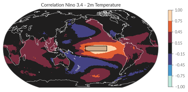
Teleconnections describe the influence of a climate oscillation on the climate of a distant region. In this section, we’ll delve into the teleconnections of ENSO on continental surface temperature, using the NINO3.4 index as a representative for the ENSO state. For this purpose, we’ll utilise the monthly averaged 2m temperature data from the ERA5 reanalysis.

A practical method to explore these teleconnections is through correlation analysis. Specifically, we’ll calculate the Pearson correlation coefficient between the NINO3.4 index and the continental surface temperatures. Typically, areas with high correlation coefficients highlight regions potentially influenced by ENSO on their surface temperatures. However, it’s crucial to remember that a strong correlation doesn’t necessarily imply a direct cause-and-effect relationship; spurious correlations may exist. For the sake of brevity and simplicity in this tutorial, we’ll treat the Pearson correlation coefficient as an initial approximation to pinpoint possible teleconnection regions. Fortunately, xarray offers a convenient built-in corr method, enabling us to conduct this analysis seamlessly in a single line of code.

corr_nino34_t2m = xr.corr(nino34, t2m, dim="time")

with ProgressBar():
    corr_nino34_t2m = corr_nino34_t2m.compute()

[########################################] | 100% Completed | 105.12 s

As a reference, let’s define a rectangular box that encompasses the NINO3.4 region.

nino34_region = dict(
    lon=[190, 240, 240, 190, 190],
    lat=[-5, -5, 5, 5, -5]
)

Now we plot the correlation coefficients together with the NINO3.4 index region.

fig = plt.figure(figsize=(8, 4))
ax = fig.add_subplot(111, projection=proj["map_global"])
corr_nino34_t2m.plot(ax=ax, transform=proj["data"], cmap="icefire", vmin=-1, vmax=1, levels=[-1, -.75, -.45, -.15, .15, .45, .75, 1], cbar_kwargs={"shrink": 0.8})
ax.coastlines(lw=.5, color="w")
# Add Nino 3.4 region
ax.plot(nino34_region["lon"], nino34_region["lat"], transform=proj["data"], color="k", lw=1)
ax.fill(nino34_region["lon"], nino34_region["lat"], transform=proj["data"], color="k", alpha=0.2)
ax.set_title("Correlation Nino 3.4 - 2m Temperature", loc="center")
plt.show()

NAO Index

The North Atlantic Oscillation (NAO) is a significant fluctuation in atmospheric pressure between the subtropical high-pressure system near the Azores in the Atlantic Ocean and the sub-polar low-pressure system near Iceland. It’s a pivotal determinant of winter climate patterns in Europe. The NAO quantifies the strength of the westerly winds over the North Atlantic. While numerous ways exist to define the NAO index, the variations between them are generally slight.

In this section, we’ll adopt the definition found in the ESOTC 2022.

Succinctly, the NAO index is computed as follows:

1. Empirical Orthogonal Function (EOF) analysis is conducted on daily area-weighted 500 hPa geopotential height (Z500) anomalies from the ERA5 reanalysis covering the Euro-Atlantic region (30°N to 88.5°N, 80°W to 40°E) from 1980–2008. Only data from October–April are utilised in this phase. The NAO pattern is characterised by the first mode derived from this EOF analysis.

2. A daily NAO index time series is then produced by projecting the daily Z500 anomalies from ERA5 onto the NAO pattern established in the first step. This series is subsequently standardised using its standard deviation from 1991–2020. Notably, the daily anomalies deployed in the second step are deduced from the daily climatology spanning 1991–2020.

Info:
For ESOTC 2022, the ERA-Interim dataset is used instead of ERA5.

Downloading the Data

To suppress the output, we instantiate a new cdsapi Client.

c = cdsapi.Client(quiet=True, progress=False)

Given our intent to fetch daily data, it’s prudent to cluster months in batches, enhancing the download efficiency. Thus, we designate the years and months for download.

YEARS = ["{:04d}".format(y) for y in range(1970, 2022)]
MONTHS = ["{:02d}".format(m) for m in range(1, 13)]

The CDS hosts an application allowing daily ERA5 statistics derivation. A comprehensive manual on this application’s operation can be found here.

Warning:
The upcoming cell will download approximately 9 GB. Ensure you have sufficient storage space. Depending on your internet speed, this could take several hours.

for year in tqdm(YEARS, desc="Overall progress"):
    for month in tqdm(MONTHS, desc="Year {}".format(year), leave=False):
        # Define the filename and the path to save the file
        path_to_file = f"data/gph/era5_z500_{year}_{month}.nc"
        # Check if the extracted files already exist
        file_exits = os.path.exists(path_to_file)
        # Download the file only if it doesn"t exist
        if not file_exits:
            result = c.service(
                "tool.toolbox.orchestrator.workflow",
                params={
                    "realm": "user-apps",
                    "project": "app-c3s-daily-era5-statistics",
                    "version": "master",
                    "kwargs": {
                        "dataset": "reanalysis-era5-pressure-levels",
                        "product_type": "reanalysis",
                        "variable": "geopotential",
                        "statistic": "daily_mean",
                        "year": year,
                        "month": month,
                        "time_zone": "UTC+00:00",
                        "frequency": "1-hourly",
                        "grid": "0.25/0.25",
                        "pressure_level": "500",
                        "area": {"lat": [30, 88.5], "lon": [-80, 40]}
                    },
                    "workflow_name": "application"
            })
            c.download(result, targets=[path_to_file])

Next, we access the data:

z500 = xr.open_mfdataset("data/gph/*.nc")
z500

<xarray.Dataset>
Dimensions:      (time: 19358, lat: 235, lon: 481)
Coordinates:
  * time         (time) datetime64[ns] 1970-01-01 1970-01-02 ... 2022-12-31
    realization  int64 0
    plev         float64 5e+04
  * lat          (lat) float64 30.0 30.25 30.5 30.75 ... 87.75 88.0 88.25 88.5
  * lon          (lon) float64 -80.0 -79.75 -79.5 -79.25 ... 39.5 39.75 40.0
Data variables:
    z            (time, lat, lon) float32 dask.array<chunksize=(31, 235, 481), meta=np.ndarray>
Attributes:
    Conventions:  CF-1.7
    institution:  European Centre for Medium-Range Weather Forecasts
    history:      2023-09-13T15:03 GRIB to CDM+CF via cfgrib-0.9.9.1/ecCodes-...
    source:       ECMWF

xarray.Dataset

• Dimensions:
  • time: 19358
  • lat: 235
  • lon: 481
• Coordinates: (5)
  • time
    (time)
    datetime64[ns]
    1970-01-01 ... 2022-12-31

    long_name :

    time

    standard_name :

    time

    axis :

    T

    stored_direction :

    increasing

    type :

    double

    array(['1970-01-01T00:00:00.000000000', '1970-01-02T00:00:00.000000000',
           '1970-01-03T00:00:00.000000000', ..., '2022-12-29T00:00:00.000000000',
           '2022-12-30T00:00:00.000000000', '2022-12-31T00:00:00.000000000'],
          dtype='datetime64[ns]')

  • realization
    ()
    int64
    0

    long_name :

    realization

    units :

    1

    standard_name :

    realization

    stored_direction :

    increasing

    type :

    integer

    array(0)

  • plev
    ()
    float64
    5e+04

    long_name :

    pressure

    units :

    Pa

    positive :

    down

    stored_direction :

    decreasing

    standard_name :

    air_pressure

    axis :

    Z

    type :

    double

    array(50000.)

  • lat
    (lat)
    float64
    30.0 30.25 30.5 ... 88.0 88.25 88.5

    units :

    degrees_north

    standard_name :

    latitude

    long_name :

    latitude

    stored_direction :

    decreasing

    axis :

    Y

    positive :

    up

    type :

    double

    valid_max :

    90.0

    valid_min :

    -90.0

    array([30.  , 30.25, 30.5 , ..., 88.  , 88.25, 88.5 ])

  • lon
    (lon)
    float64
    -80.0 -79.75 -79.5 ... 39.75 40.0

    units :

    degrees_east

    standard_name :

    longitude

    long_name :

    longitude

    axis :

    X

    positive :

    up

    type :

    double

    valid_max :

    360.0

    valid_min :

    -180.0

    array([-80.  , -79.75, -79.5 , ...,  39.5 ,  39.75,  40.  ])

• Data variables: (1)
  • z
    (time, lat, lon)
    float32
    dask.array<chunksize=(31, 235, 481), meta=np.ndarray>

    long_name :

    Geopotential

    units :

    m2 s-2

    standard_name :

    geopotential

    comment :

    Geopotential is the sum of the specific gravitational potential energy relative to the geoid and the specific centripetal potential energy.

    cds_magics_style_name :

    turbo_1000_3000

    type :

    real

    Array Chunk Bytes 8.15 GiB 13.37 MiB Shape (19358, 235, 481) (31, 235, 481) Dask graph 636 chunks in 1273 graph layers Data type float32 numpy.ndarray

• Indexes: (3)
  • time
    PandasIndex

    PandasIndex(DatetimeIndex(['1970-01-01', '1970-01-02', '1970-01-03', '1970-01-04',
                   '1970-01-05', '1970-01-06', '1970-01-07', '1970-01-08',
                   '1970-01-09', '1970-01-10',
                   ...
                   '2022-12-22', '2022-12-23', '2022-12-24', '2022-12-25',
                   '2022-12-26', '2022-12-27', '2022-12-28', '2022-12-29',
                   '2022-12-30', '2022-12-31'],
                  dtype='datetime64[ns]', name='time', length=19358, freq=None))

  • lat
    PandasIndex

    PandasIndex(Float64Index([ 30.0, 30.25,  30.5, 30.75,  31.0, 31.25,  31.5, 31.75,  32.0,
                  32.25,
                  ...
                  86.25,  86.5, 86.75,  87.0, 87.25,  87.5, 87.75,  88.0, 88.25,
                   88.5],
                 dtype='float64', name='lat', length=235))

  • lon
    PandasIndex

    PandasIndex(Float64Index([ -80.0, -79.75,  -79.5, -79.25,  -79.0, -78.75,  -78.5, -78.25,
                   -78.0, -77.75,
                  ...
                   37.75,   38.0,  38.25,   38.5,  38.75,   39.0,  39.25,   39.5,
                   39.75,   40.0],
                 dtype='float64', name='lon', length=481))

• Attributes: (4)

  Conventions :

  CF-1.7

  institution :

  European Centre for Medium-Range Weather Forecasts

  history :

  2023-09-13T15:03 GRIB to CDM+CF via cfgrib-0.9.9.1/ecCodes-2.27.0 with {"source": "/nfs/compute-0018/data9/adaptor.mars.internal-1694617383.266881-4329-7-c6153a93-bac4-4bb8-9b38-e2f54805658b.grib", "filter_by_keys": {}, "encode_cf": ["parameter", "time", "geography", "vertical"]}

  source :

  ECMWF

With just a singular variable at our disposal, it’s straightforward to isolate it and utilise the relevant xarray.DataArray.

z500 = z500['z']
z500

<xarray.DataArray 'z' (time: 19358, lat: 235, lon: 481)>
dask.array<concatenate, shape=(19358, 235, 481), dtype=float32, chunksize=(31, 235, 481), chunktype=numpy.ndarray>
Coordinates:
  * time         (time) datetime64[ns] 1970-01-01 1970-01-02 ... 2022-12-31
    realization  int64 0
    plev         float64 5e+04
  * lat          (lat) float64 30.0 30.25 30.5 30.75 ... 87.75 88.0 88.25 88.5
  * lon          (lon) float64 -80.0 -79.75 -79.5 -79.25 ... 39.5 39.75 40.0
Attributes:
    long_name:              Geopotential
    units:                  m2 s-2
    standard_name:          geopotential
    comment:                Geopotential is the sum of the specific gravitati...
    cds_magics_style_name:  turbo_1000_3000
    type:                   real

xarray.DataArray

'z'

• time: 19358
• lat: 235
• lon: 481

• dask.array<chunksize=(31, 235, 481), meta=np.ndarray>

  Array Chunk Bytes 8.15 GiB 13.37 MiB Shape (19358, 235, 481) (31, 235, 481) Dask graph 636 chunks in 1273 graph layers Data type float32 numpy.ndarray

• Coordinates: (5)
  • time
    (time)
    datetime64[ns]
    1970-01-01 ... 2022-12-31

    long_name :

    time

    standard_name :

    time

    axis :

    T

    stored_direction :

    increasing

    type :

    double

    array(['1970-01-01T00:00:00.000000000', '1970-01-02T00:00:00.000000000',
           '1970-01-03T00:00:00.000000000', ..., '2022-12-29T00:00:00.000000000',
           '2022-12-30T00:00:00.000000000', '2022-12-31T00:00:00.000000000'],
          dtype='datetime64[ns]')

  • realization
    ()
    int64
    0

    long_name :

    realization

    units :

    1

    standard_name :

    realization

    stored_direction :

    increasing

    type :

    integer

    array(0)

  • plev
    ()
    float64
    5e+04

    long_name :

    pressure

    units :

    Pa

    positive :

    down

    stored_direction :

    decreasing

    standard_name :

    air_pressure

    axis :

    Z

    type :

    double

    array(50000.)

  • lat
    (lat)
    float64
    30.0 30.25 30.5 ... 88.0 88.25 88.5

    units :

    degrees_north

    standard_name :

    latitude

    long_name :

    latitude

    stored_direction :

    decreasing

    axis :

    Y

    positive :

    up

    type :

    double

    valid_max :

    90.0

    valid_min :

    -90.0

    array([30.  , 30.25, 30.5 , ..., 88.  , 88.25, 88.5 ])

  • lon
    (lon)
    float64
    -80.0 -79.75 -79.5 ... 39.75 40.0

    units :

    degrees_east

    standard_name :

    longitude

    long_name :

    longitude

    axis :

    X

    positive :

    up

    type :

    double

    valid_max :

    360.0

    valid_min :

    -180.0

    array([-80.  , -79.75, -79.5 , ...,  39.5 ,  39.75,  40.  ])

• Indexes: (3)
  • time
    PandasIndex

    PandasIndex(DatetimeIndex(['1970-01-01', '1970-01-02', '1970-01-03', '1970-01-04',
                   '1970-01-05', '1970-01-06', '1970-01-07', '1970-01-08',
                   '1970-01-09', '1970-01-10',
                   ...
                   '2022-12-22', '2022-12-23', '2022-12-24', '2022-12-25',
                   '2022-12-26', '2022-12-27', '2022-12-28', '2022-12-29',
                   '2022-12-30', '2022-12-31'],
                  dtype='datetime64[ns]', name='time', length=19358, freq=None))

  • lat
    PandasIndex

    PandasIndex(Float64Index([ 30.0, 30.25,  30.5, 30.75,  31.0, 31.25,  31.5, 31.75,  32.0,
                  32.25,
                  ...
                  86.25,  86.5, 86.75,  87.0, 87.25,  87.5, 87.75,  88.0, 88.25,
                   88.5],
                 dtype='float64', name='lat', length=235))

  • lon
    PandasIndex

    PandasIndex(Float64Index([ -80.0, -79.75,  -79.5, -79.25,  -79.0, -78.75,  -78.5, -78.25,
                   -78.0, -77.75,
                  ...
                   37.75,   38.0,  38.25,   38.5,  38.75,   39.0,  39.25,   39.5,
                   39.75,   40.0],
                 dtype='float64', name='lon', length=481))

• Attributes: (6)

  long_name :

  Geopotential

  units :

  m2 s-2

  standard_name :

  geopotential

  comment :

  Geopotential is the sum of the specific gravitational potential energy relative to the geoid and the specific centripetal potential energy.

  cds_magics_style_name :

  turbo_1000_3000

  type :

  real

Computing Daily Anomalies

The initial task for computing daily anomalies is establishing the daily climatology. The predefined reference period (1991-2020) will serve as our benchmark.

daily_climatoloy = z500.sel(REF_PERIOD).groupby("time.dayofyear").mean()
with ProgressBar():
    daily_climatoloy = daily_climatoloy.compute()

[########################################] | 100% Completed | 41.90 s

We can now proceed to calculate the daily anomalies.

z500_anomalies = z500.groupby("time.dayofyear") - daily_climatoloy

/home/nrieger/miniconda3/envs/tutorial/lib/python3.10/site-packages/xarray/core/indexing.py:1443: PerformanceWarning: Slicing with an out-of-order index is generating 53 times more chunks
  return self.array[key]

Deriving the NAO Index

As previously outlined, the NAO index is based on the first EOF mode of daily Z500 anomalies from October through April, spanning 1980 to 2008. First, we select this specific time period.

is_winter_month = z500_anomalies.time.dt.month.isin([10,11,12,1,2,3,4])
z500_nao_ref = z500_anomalies.isel(time=is_winter_month).sel(time=slice("1980-01-01", "2008-12-31"))
z500_nao_ref

/home/nrieger/miniconda3/envs/tutorial/lib/python3.10/site-packages/xarray/core/accessor_dt.py:72: FutureWarning: Index.ravel returning ndarray is deprecated; in a future version this will return a view on self.
  values_as_series = pd.Series(values.ravel(), copy=False)

<xarray.DataArray 'z' (time: 6156, lat: 235, lon: 481)>
dask.array<getitem, shape=(6156, 235, 481), dtype=float32, chunksize=(1, 235, 481), chunktype=numpy.ndarray>
Coordinates:
  * time         (time) datetime64[ns] 1980-01-01 1980-01-02 ... 2008-12-31
    realization  (time) int64 0 0 0 0 0 0 0 0 0 0 0 0 ... 0 0 0 0 0 0 0 0 0 0 0
    plev         (time) float64 5e+04 5e+04 5e+04 5e+04 ... 5e+04 5e+04 5e+04
  * lat          (lat) float64 30.0 30.25 30.5 30.75 ... 87.75 88.0 88.25 88.5
  * lon          (lon) float64 -80.0 -79.75 -79.5 -79.25 ... 39.5 39.75 40.0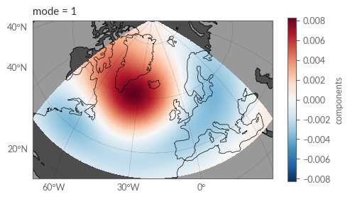
    dayofyear    (time) int64 1 2 3 4 5 6 7 8 ... 360 361 362 363 364 365 366

xarray.DataArray

'z'

• time: 6156
• lat: 235
• lon: 481

• dask.array<chunksize=(1, 235, 481), meta=np.ndarray>

  Array Chunk Bytes 2.59 GiB 441.54 kiB Shape (6156, 235, 481) (1, 235, 481) Dask graph 6156 chunks in 1279 graph layers Data type float32 numpy.ndarray

• Coordinates: (6)
  • time
    (time)
    datetime64[ns]
    1980-01-01 ... 2008-12-31

    long_name :

    time

    standard_name :

    time

    axis :

    T

    stored_direction :

    increasing

    type :

    double

    array(['1980-01-01T00:00:00.000000000', '1980-01-02T00:00:00.000000000',
           '1980-01-03T00:00:00.000000000', ..., '2008-12-29T00:00:00.000000000',
           '2008-12-30T00:00:00.000000000', '2008-12-31T00:00:00.000000000'],
          dtype='datetime64[ns]')

  • realization
    (time)
    int64
    0 0 0 0 0 0 0 0 ... 0 0 0 0 0 0 0 0

    long_name :

    realization

    units :

    1

    standard_name :

    realization

    stored_direction :

    increasing

    type :

    integer

    array([0, 0, 0, ..., 0, 0, 0])

  • plev
    (time)
    float64
    5e+04 5e+04 5e+04 ... 5e+04 5e+04

    long_name :

    pressure

    units :

    Pa

    positive :

    down

    stored_direction :

    decreasing

    standard_name :

    air_pressure

    axis :

    Z

    type :

    double

    array([50000., 50000., 50000., ..., 50000., 50000., 50000.])

  • lat
    (lat)
    float64
    30.0 30.25 30.5 ... 88.0 88.25 88.5

    units :

    degrees_north

    standard_name :

    latitude

    long_name :

    latitude

    stored_direction :

    decreasing

    axis :

    Y

    positive :

    up

    type :

    double

    valid_max :

    90.0

    valid_min :

    -90.0

    array([30.  , 30.25, 30.5 , ..., 88.  , 88.25, 88.5 ])

  • lon
    (lon)
    float64
    -80.0 -79.75 -79.5 ... 39.75 40.0

    units :

    degrees_east

    standard_name :

    longitude

    long_name :

    longitude

    axis :

    X

    positive :

    up

    type :

    double

    valid_max :

    360.0

    valid_min :

    -180.0

    array([-80.  , -79.75, -79.5 , ...,  39.5 ,  39.75,  40.  ])

  • dayofyear
    (time)
    int64
    1 2 3 4 5 6 ... 362 363 364 365 366

    array([  1,   2,   3, ..., 364, 365, 366])

• Indexes: (3)
  • time
    PandasIndex

    PandasIndex(DatetimeIndex(['1980-01-01', '1980-01-02', '1980-01-03', '1980-01-04',
                   '1980-01-05', '1980-01-06', '1980-01-07', '1980-01-08',
                   '1980-01-09', '1980-01-10',
                   ...
                   '2008-12-22', '2008-12-23', '2008-12-24', '2008-12-25',
                   '2008-12-26', '2008-12-27', '2008-12-28', '2008-12-29',
                   '2008-12-30', '2008-12-31'],
                  dtype='datetime64[ns]', name='time', length=6156, freq=None))

  • lat
    PandasIndex

    PandasIndex(Float64Index([ 30.0, 30.25,  30.5, 30.75,  31.0, 31.25,  31.5, 31.75,  32.0,
                  32.25,
                  ...
                  86.25,  86.5, 86.75,  87.0, 87.25,  87.5, 87.75,  88.0, 88.25,
                   88.5],
                 dtype='float64', name='lat', length=235))

  • lon
    PandasIndex

    PandasIndex(Float64Index([ -80.0, -79.75,  -79.5, -79.25,  -79.0, -78.75,  -78.5, -78.25,
                   -78.0, -77.75,
                  ...
                   37.75,   38.0,  38.25,   38.5,  38.75,   39.0,  39.25,   39.5,
                   39.75,   40.0],
                 dtype='float64', name='lon', length=481))

• Attributes: (0)

The next step involves conducting the EOF analysis using the xeofs package. To initialise the EOF model, we need to specify the number of modes to compute. As we’re primarily interested in the first mode, we set this value to 1. We also have to weight the individual grid cells to account for the convergence of the meridians the poles which we do by setting the use_coslat parameter to True.

eof_model = xe.models.EOF(n_modes=1, use_coslat=True)

Next, we simply fit the model to our data. Crucially, we need to specify the dimension for the EOF analysis, which in our case is the time dimension.

eof_model.fit(z500_nao_ref, dim="time")

Post this, we can capture the EOF pattern and the affiliated principal component (PC). Given our input was sourced from dask arrays, both the EOF pattern and PC echo this format. Prior to visualisation, we therefore need to compute the results. Thankfully, xeofs furnishes a useful method, computing all results simultaneously.

eof_model.compute(verbose=True)

[########################################] | 100% Completed | 11m 41s
[########################################] | 100% Completed | 10m 48s
[########################################] | 100% Completed | 11m 37s
[########################################] | 100% Completed | 75.40 s

Subsequently, we extract the spatial patterns (components).

components = eof_model.components()

Examining the first EOF mode of the Z500 anomalies reveals the evident NAO pattern. Note, however, that the sign of the pattern is inverse to the NAO pattern typically presented in literature. This is because the EOF analysis is agnostic to the sign of the pattern. Thus, we can simply flip the sign of the pattern to match the conventional NAO pattern.

fig = plt.figure(figsize=(12, 3))
ax = fig.add_subplot(121, projection=proj["map_north_atlantic"])
ax.coastlines(lw=.5)
ax.add_feature(cfeature.LAND, color=".6")
ax.add_feature(cfeature.OCEAN, color=".3")
gl = ax.gridlines(draw_labels=True, color='.1', ls=':', lw=.25)
gl.top_labels = False
gl.right_labels = False
components.sel(mode=1).plot(transform=ccrs.PlateCarree(), ax=ax)
plt.show()

In the following step, the NAO index’s daily time series is obtained by projecting the ERA5 daily Z500 anomalies onto the previously delineated NAO pattern. This projection is executed via the transform method within the xeofs model.

pseudo_pcs = eof_model.transform(z500_anomalies)

The first mode, embodying the NAO index, is selected. As mentioned before, we flip the sign of the index to match the conventional NAO index definition.

nao_index = -pseudo_pcs.sel(mode=1)

We compute the NAO index.

with ProgressBar():
    nao_index = nao_index.compute()

[########################################] | 100% Completed | 98.63 s

The concluding step entails standardising the NAO index using its 1991–2020 standard deviation.

nao_index = nao_index / nao_index.sel(REF_PERIOD).std("time")

Time to visualise the NAO index. To echo the ESOTC 2022’s depiction, we craft a helper function positioning the labels aptly between the x-ticks.

def center_labels_between_xticks(ax):
    # set y-ticks as integers
    ax.yaxis.set_major_locator(ticker.MaxNLocator(integer=True))

    # Set major x-ticks every 1 month
    ax.xaxis.set_major_locator(dates.MonthLocator())


    # Centering labels between ticks
    # 16 is a slight approximation since months differ in number of days.
    ax.xaxis.set_minor_locator(dates.MonthLocator(bymonthday=16))
    ax.xaxis.set_major_formatter(ticker.NullFormatter())
    ax.xaxis.set_minor_formatter(dates.DateFormatter("%b"))

    # Remove the minor tick lines
    ax.tick_params(axis="x", which="minor", tick1On=False, tick2On=False)

    # Align the minor tick label
    for label in ax.get_xticklabels(minor=True):
        label.set_horizontalalignment("center")

Moreover, a 7-day rolling mean is applied, lending a smoother edge to the NAO index.

nao_index_smooth = nao_index.rolling(time=7, center=True).mean()

Lastly, we plot the NAO index.

year = 2022

fig, ax = plt.subplots(figsize=(10, 2))
ax.fill_between(nao_index_smooth.time, 0, nao_index_smooth, where=nao_index_smooth >= 0, color="red", alpha=0.5)
ax.fill_between(nao_index_smooth.time, 0, nao_index_smooth, where=nao_index_smooth <= 0, color="blue", alpha=0.5)
ax.axhline(0, color="k", linewidth=0.5)
ax.set_title("North Atlantic Osciallation (NAO) Index - {}".format(year))
ax.set_ylabel("")
ax.set_xlabel("")
ax.set_ylim(-3, 3)

xlim1 = dt.datetime.strptime(f"{year}-01-01", "%Y-%m-%d")
xlim2 = dt.datetime.strptime(f"{year}-12-31", "%Y-%m-%d")
ax.set_xlim(xlim1, xlim2)
center_labels_between_xticks(ax)
sns.despine(ax=ax, offset=10)

Note:
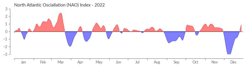
Looking carefully you will spot minor differences between the NAO index presented here and the one in the ESOTC 2022. This is due to the usage of ERA-Interim in the ESOTC 2022 for defining the NAO pattern instead of ERA5.

Conclusion

This tutorial illuminated the process of extracting both the ENSO and NAO indices from ERA5 data. We also touched upon the methodology of investigating teleconnections, demonstrated with an surface temperature teleconnections of ENSO.